
Creating your first population#
Welcome to the cogsworth tutorials! In this tutorial we will create a simple population of binaries.
Learning Goals#
By the end of this tutorial you should know:
What the
Populationclass can doHow to initialise a simple
PopulationHow to create a full population with basic settings using
create_population()
[1]:
import cogsworth
import gala.potential as gp
import astropy.units as u
import matplotlib.pyplot as plt
import numpy as np
[2]:
# this all just makes plots look nice
%config InlineBackend.figure_format = 'retina'

plt.rc('font', family='serif')
plt.rcParams['text.usetex'] = False
fs = 24

# update various fontsizes to match
params = {'figure.figsize': (12, 8),
          'legend.fontsize': fs,
          'axes.labelsize': fs,
          'xtick.labelsize': 0.9 * fs,
          'ytick.labelsize': 0.9 * fs,
          'axes.linewidth': 1.1,
          'xtick.major.size': 7,
          'xtick.minor.size': 4,
          'ytick.major.size': 7,
          'ytick.minor.size': 4}
plt.rcParams.update(params)
The Population Class#
The core functionality of cogsworth is to simulate populations of binaries in the context of the galaxy.
This is implemented primarily through the Population class, which will give you access
to the vast majority of cogsworth’s features.
Let’s initialise a simple population of binaries using the default input settings:
[3]:
p = cogsworth.pop.Population(n_binaries=100, processes=4,
                             final_kstar1=list(range(16)), final_kstar2=list(range(16)),
                             sfh_model=cogsworth.sfh.Wagg2022(),
                             galactic_potential=gp.MilkyWayPotential(version='v2'),
                             v_dispersion=5 * u.km / u.s,
                             max_ev_time=12.0 * u.Gyr, timestep_size=1 * u.Myr,
                             BSE_settings={}, sampling_params={}, store_entire_orbits=True,
                             use_default_BSE_settings=True)
Basic input settings#
The Population class has a number of input settings that can be used to control the way
in which the population is created. Many of these directly affect the way in which a population is evolved or
the initial conditions are sampled and these are covered in later tutorials.
For now, we will focus on the basic settings:
n_binaries: By default,cogsworthsamples a population by targetting a number of binaries, this is that target valueprocesses: This is the number of CPUs to use for the population, which uses a multiprocessing pool for a variety of tasks. In general, the speed of the simulation scales with the number of processors.max_ev_time: How long to evolve a simulation for
The rest of the settings will be addressed in those other tutorials. Try running the next part with different values for these parameters and seeing what happens
Creating a population#
The manual way#
First let’s look a how you create a population manually, step-by-step (which can be useful for custom populations later on!).
[4]:
p = cogsworth.pop.Population(n_binaries=1000, processes=4, max_ev_time=12.0 * u.Gyr,
                             use_default_BSE_settings=True)
Initial stellar population#
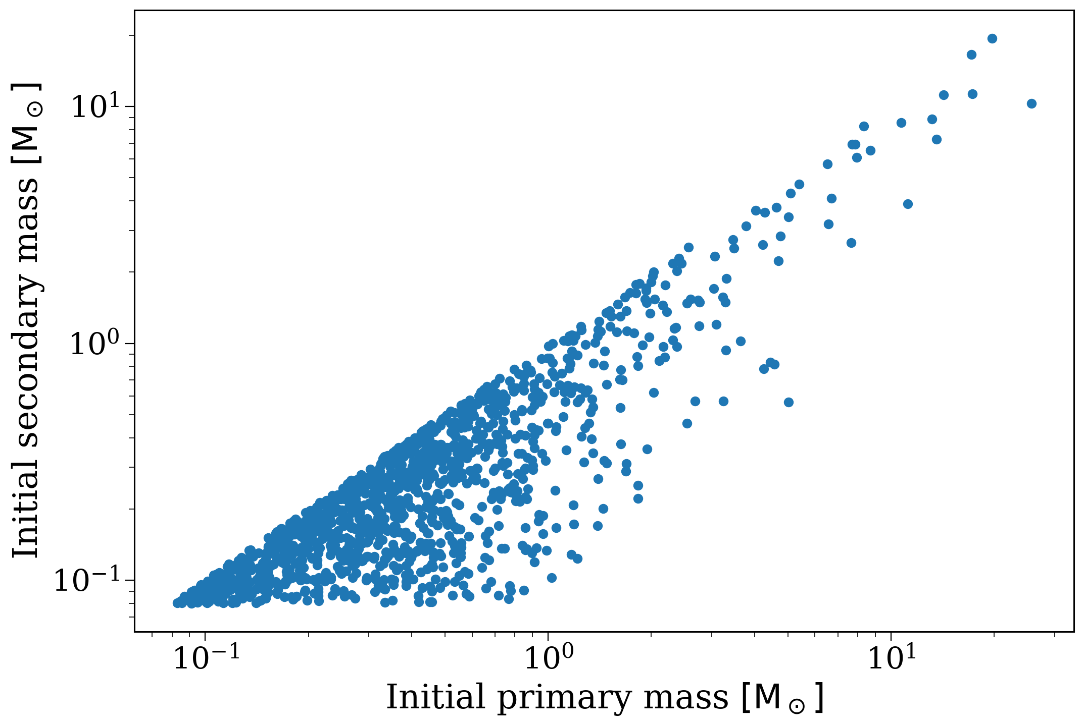
Let’s start by sampling initial stellar population. This will create the _initial_binaries table as well as store values for the mass_singles, mass_binaries, n_singles_req, n_bin_req, which track the mass and number of single stars and binary stars necessary to sample this population.
Check out the sampling tutorial for more info and changing the sampling settings.
[5]:
# now let's get the initital stellar population
p.sample_initial_binaries()
p._initial_binaries
[5]:
| kstar_1 | kstar_2 | mass_1 | mass_2 | porb | ecc | metallicity | tphysf | mass0_1 | mass0_2 | ... | tacc_1 | tacc_2 | epoch_1 | epoch_2 | tms_1 | tms_2 | bhspin_1 | bhspin_2 | tphys | binfrac | |
|---|---|---|---|---|---|---|---|---|---|---|---|---|---|---|---|---|---|---|---|---|---|
| 0 | 0.0 | 0.0 | 0.315141 | 0.237802 | 4.707982 | 0.848973 | 0.027476 | 3757.812769 | 0.315141 | 0.237802 | ... | 0.0 | 0.0 | 0.0 | 0.0 | 0.0 | 0.0 | 0.0 | 0.0 | 0.0 | 1.0 |
| 1 | 0.0 | 0.0 | 0.231263 | 0.151861 | 74444.055334 | 0.616752 | 0.030000 | 3414.805657 | 0.231263 | 0.151861 | ... | 0.0 | 0.0 | 0.0 | 0.0 | 0.0 | 0.0 | 0.0 | 0.0 | 0.0 | 1.0 |
| 2 | 1.0 | 0.0 | 0.748870 | 0.569088 | 1137.259444 | 0.006560 | 0.007444 | 7956.431410 | 0.748870 | 0.569088 | ... | 0.0 | 0.0 | 0.0 | 0.0 | 0.0 | 0.0 | 0.0 | 0.0 | 0.0 | 1.0 |
| 3 | 0.0 | 0.0 | 0.255084 | 0.085582 | 5.973114 | 0.025460 | 0.001126 | 2194.571045 | 0.255084 | 0.085582 | ... | 0.0 | 0.0 | 0.0 | 0.0 | 0.0 | 0.0 | 0.0 | 0.0 | 0.0 | 1.0 |
| 4 | 0.0 | 0.0 | 0.273239 | 0.250952 | 1893.639998 | 0.037405 | 0.016313 | 976.319501 | 0.273239 | 0.250952 | ... | 0.0 | 0.0 | 0.0 | 0.0 | 0.0 | 0.0 | 0.0 | 0.0 | 0.0 | 1.0 |
| ... | ... | ... | ... | ... | ... | ... | ... | ... | ... | ... | ... | ... | ... | ... | ... | ... | ... | ... | ... | ... | ... |
| 1299 | 1.0 | 0.0 | 0.709939 | 0.376113 | 53.269380 | 0.314557 | 0.011130 | 9214.340705 | 0.709939 | 0.376113 | ... | 0.0 | 0.0 | 0.0 | 0.0 | 0.0 | 0.0 | 0.0 | 0.0 | 0.0 | 1.0 |
| 1300 | 1.0 | 0.0 | 1.169294 | 0.128767 | 89.504234 | 0.019073 | 0.019907 | 6821.312805 | 1.169294 | 0.128767 | ... | 0.0 | 0.0 | 0.0 | 0.0 | 0.0 | 0.0 | 0.0 | 0.0 | 0.0 | 1.0 |
| 1301 | 0.0 | 0.0 | 0.128548 | 0.117100 | 3.499193 | 0.214564 | 0.006029 | 7401.934328 | 0.128548 | 0.117100 | ... | 0.0 | 0.0 | 0.0 | 0.0 | 0.0 | 0.0 | 0.0 | 0.0 | 0.0 | 1.0 |
| 1302 | 0.0 | 0.0 | 0.391459 | 0.386078 | 196.105254 | 0.039243 | 0.009519 | 9160.456454 | 0.391459 | 0.386078 | ... | 0.0 | 0.0 | 0.0 | 0.0 | 0.0 | 0.0 | 0.0 | 0.0 | 0.0 | 1.0 |
| 1303 | 0.0 | 0.0 | 0.091023 | 0.089575 | 139.850990 | 0.028575 | 0.008901 | 9012.216598 | 0.091023 | 0.089575 | ... | 0.0 | 0.0 | 0.0 | 0.0 | 0.0 | 0.0 | 0.0 | 0.0 | 0.0 | 1.0 |
1304 rows × 38 columns
[6]:
fig, ax = plt.subplots()
ax.scatter(p._initial_binaries["mass_1"], p._initial_binaries["mass_2"])
ax.set(xscale="log", yscale="log",
       xlabel=r"Initial primary mass $[\rm M_\odot]$", ylabel=r"Initial secondary mass $[\rm M_\odot]$")
plt.show()
Initial galaxy sampling#
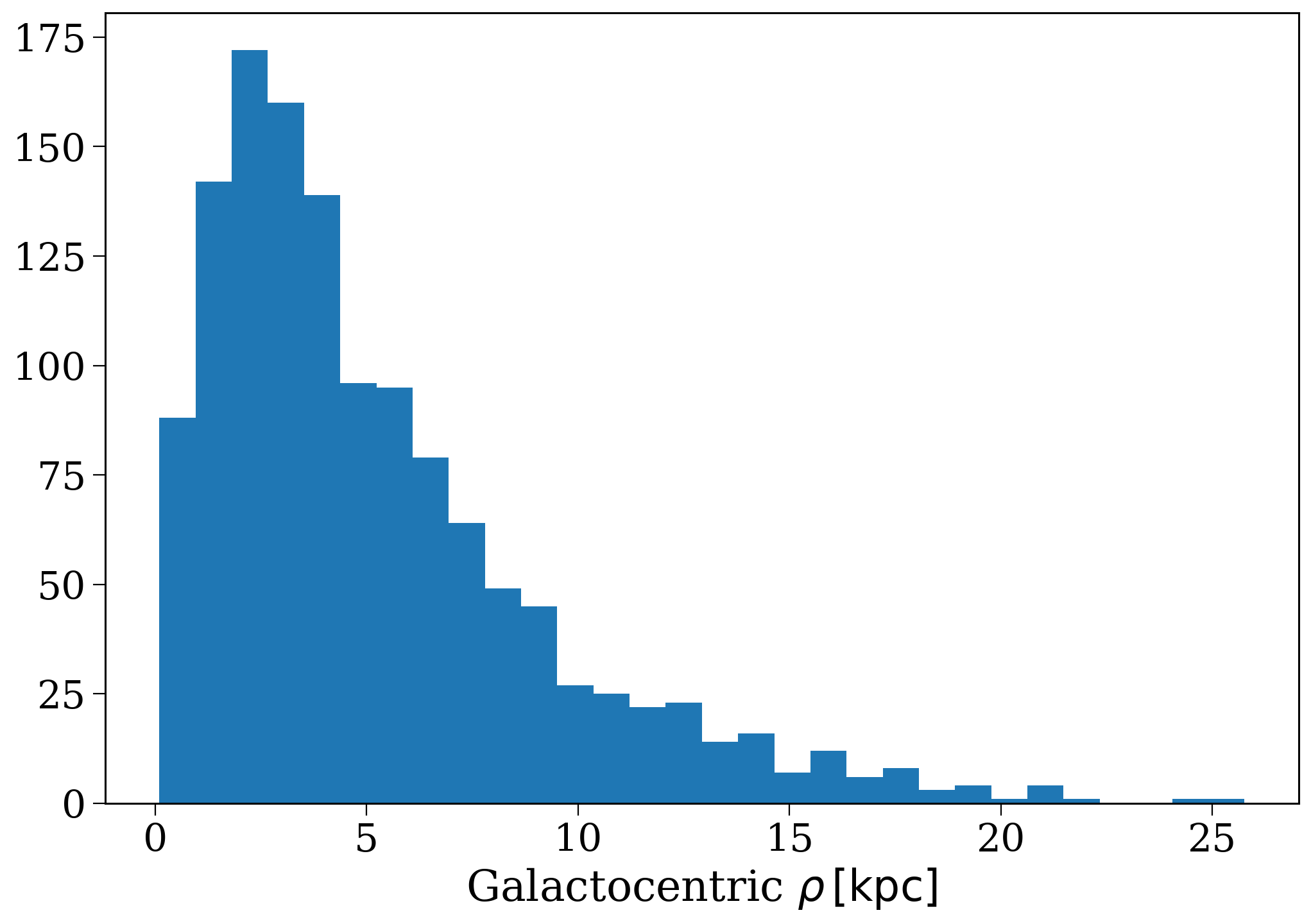
Now let’s try sampling the initial galactic positions, kinematics and birth times. This will create the initial_galaxy attribute, which is a Galaxy that was instantiated based on your input choice of sfh_model when creating the Population.
Check out the star formation history tutorial for more info and changing initial galaxy sampling settings.
[7]:
# first let's sample the initial galaxy
p.sample_initial_galaxy()

# and check distributions look normal
plt.hist(p.initial_galaxy.rho.value, bins="fd");
plt.xlabel(r"Galactocentric $\rho \, [\rm kpc]$");
Stellar evolution#
Now we can use COSMIC to evolve the stellar population from birth until present day. This will create a series of output tables: initC (the initial conditions for each binary), bpp (the evolution table each binary), bcm (the conditioned timestep evolution table for each binary) and kick_info (the kicks experienced by each binary).
Check out this tutorial for more info and changing the population synthesis settings.
[8]:
p.perform_stellar_evolution()
p.bpp
[8]:
| tphys | mass_1 | mass_2 | kstar_1 | kstar_2 | sep | porb | ecc | RRLO_1 | RRLO_2 | ... | B_2 | bacc_1 | bacc_2 | tacc_1 | tacc_2 | epoch_1 | epoch_2 | bhspin_1 | bhspin_2 | bin_num | |
|---|---|---|---|---|---|---|---|---|---|---|---|---|---|---|---|---|---|---|---|---|---|
| 0 | 0.000000 | 0.315141 | 0.237802 | 0 | 0 | 9.699181 | 4.707982 | 0.848973 | 0.541792 | 0.512880 | ... | 0.0 | 0.0 | 0.0 | 0.0 | 0.0 | 0.0 | 0.0 | 0.0 | 0.0 | 0 |
| 0 | 3757.812769 | 0.315141 | 0.237802 | 0 | 0 | 6.642473 | 2.668253 | 0.779200 | 0.541947 | 0.512688 | ... | 0.0 | 0.0 | 0.0 | 0.0 | 0.0 | 0.0 | 0.0 | 0.0 | 0.0 | 0 |
| 1 | 0.000000 | 0.231263 | 0.151861 | 0 | 0 | 5406.942159 | 74444.055334 | 0.616752 | 0.000306 | 0.000276 | ... | 0.0 | 0.0 | 0.0 | 0.0 | 0.0 | 0.0 | 0.0 | 0.0 | 0.0 | 1 |
| 1 | 3414.805657 | 0.231263 | 0.151861 | 0 | 0 | 5406.942159 | 74444.055334 | 0.616752 | 0.000306 | 0.000276 | ... | 0.0 | 0.0 | 0.0 | 0.0 | 0.0 | 0.0 | 0.0 | 0.0 | 0.0 | 1 |
| 2 | 0.000000 | 0.748870 | 0.569088 | 1 | 0 | 502.526231 | 1137.259444 | 0.006560 | 0.003441 | 0.002959 | ... | 0.0 | 0.0 | 0.0 | 0.0 | 0.0 | 0.0 | 0.0 | 0.0 | 0.0 | 2 |
| ... | ... | ... | ... | ... | ... | ... | ... | ... | ... | ... | ... | ... | ... | ... | ... | ... | ... | ... | ... | ... | ... |
| 1301 | 7401.934328 | 0.128548 | 0.117100 | 0 | 0 | 6.072176 | 3.498911 | 0.214546 | 0.085784 | 0.081986 | ... | 0.0 | 0.0 | 0.0 | 0.0 | 0.0 | 0.0 | 0.0 | 0.0 | 0.0 | 1301 |
| 1302 | 0.000000 | 0.391459 | 0.386078 | 0 | 0 | 130.572504 | 196.105254 | 0.039243 | 0.007664 | 0.007626 | ... | 0.0 | 0.0 | 0.0 | 0.0 | 0.0 | 0.0 | 0.0 | 0.0 | 0.0 | 1302 |
| 1302 | 9160.456454 | 0.391459 | 0.386078 | 0 | 0 | 130.572503 | 196.105253 | 0.039243 | 0.007731 | 0.007691 | ... | 0.0 | 0.0 | 0.0 | 0.0 | 0.0 | 0.0 | 0.0 | 0.0 | 0.0 | 1302 |
| 1303 | 0.000000 | 0.091023 | 0.089575 | 0 | 0 | 64.066782 | 139.850990 | 0.028575 | 0.006061 | 0.006138 | ... | 0.0 | 0.0 | 0.0 | 0.0 | 0.0 | 0.0 | 0.0 | 0.0 | 0.0 | 1303 |
| 1303 | 9012.216598 | 0.091023 | 0.089575 | 0 | 0 | 64.066782 | 139.850990 | 0.028575 | 0.006061 | 0.006138 | ... | 0.0 | 0.0 | 0.0 | 0.0 | 0.0 | 0.0 | 0.0 | 0.0 | 0.0 | 1303 |
4147 rows × 46 columns
[9]:
# print out some evolution information for the most massive binary
# we'll cover more on how this masking works in the next few tutorials
p.bpp.loc[p.initial_binaries[p.initial_binaries["mass_1"] == p.initial_binaries["mass_1"].max()]["bin_num"].iloc[0]]
[9]:
| tphys | mass_1 | mass_2 | kstar_1 | kstar_2 | sep | porb | ecc | RRLO_1 | RRLO_2 | ... | B_2 | bacc_1 | bacc_2 | tacc_1 | tacc_2 | epoch_1 | epoch_2 | bhspin_1 | bhspin_2 | bin_num | |
|---|---|---|---|---|---|---|---|---|---|---|---|---|---|---|---|---|---|---|---|---|---|
| 1041 | 0.000000 | 25.642687 | 10.300848 | 1 | 1 | 24.597121 | 2.358241 | 0.019168 | 5.609188e-01 | 0.489863 | ... | 0.0 | 0.0 | 0.0 | 0.0 | 0.0 | 0.000000 | 0.000000 | 0.0 | 0.0 | 1041 |
| 1041 | 5.512373 | 25.043363 | 10.326454 | 1 | 1 | 23.603469 | 2.234701 | 0.000000 | 1.000249e+00 | 0.558423 | ... | 0.0 | 0.0 | 0.0 | 0.0 | 0.0 | -0.076161 | 0.014830 | 0.0 | 0.0 | 1041 |
| 1041 | 5.512373 | 0.000000 | 35.369817 | 15 | 1 | 0.000000 | 0.000000 | -1.000000 | 0.000000e+00 | -1.000000 | ... | 0.0 | 0.0 | 0.0 | 0.0 | 0.0 | -0.076161 | 5.148750 | 0.0 | 0.0 | 1041 |
| 1041 | 10.773904 | 0.000000 | 32.986648 | 15 | 2 | 0.000000 | 0.000000 | -1.000000 | -9.264869e-12 | 0.000100 | ... | 0.0 | 0.0 | 0.0 | 0.0 | 0.0 | -0.076161 | 4.963135 | 0.0 | 0.0 | 1041 |
| 1041 | 10.781241 | 0.000000 | 32.934501 | 15 | 4 | 0.000000 | 0.000000 | -1.000000 | -9.264869e-12 | 0.000100 | ... | 0.0 | 0.0 | 0.0 | 0.0 | 0.0 | -0.076161 | 4.963135 | 0.0 | 0.0 | 1041 |
| 1041 | 11.380735 | 0.000000 | 15.292669 | 15 | 5 | 0.000000 | 0.000000 | -1.000000 | -9.264869e-12 | 0.000100 | ... | 0.0 | 0.0 | 0.0 | 0.0 | 0.0 | -0.076161 | 4.963135 | 0.0 | 0.0 | 1041 |
| 1041 | 11.392238 | 0.000000 | 13.696400 | 15 | 5 | 0.000000 | 0.000000 | -1.000000 | -9.264869e-12 | 0.000100 | ... | 0.0 | 0.0 | 0.0 | 0.0 | 0.0 | -0.076161 | 4.963135 | 0.0 | 0.0 | 1041 |
| 1041 | 11.392238 | 0.000000 | 12.438530 | 15 | 14 | 0.000000 | 0.000000 | -1.000000 | -9.264869e-12 | 0.000100 | ... | 0.0 | 0.0 | 0.0 | 0.0 | 0.0 | -0.076161 | 11.392238 | 0.0 | 0.0 | 1041 |
| 1041 | 11080.186301 | 0.000000 | 12.438530 | 15 | 14 | 0.000000 | 0.000000 | -1.000000 | -9.264869e-12 | 0.000100 | ... | 0.0 | 0.0 | 0.0 | 0.0 | 0.0 | -0.076161 | 11.392238 | 0.0 | 0.0 | 1041 |
9 rows × 46 columns
Galactic evolution#
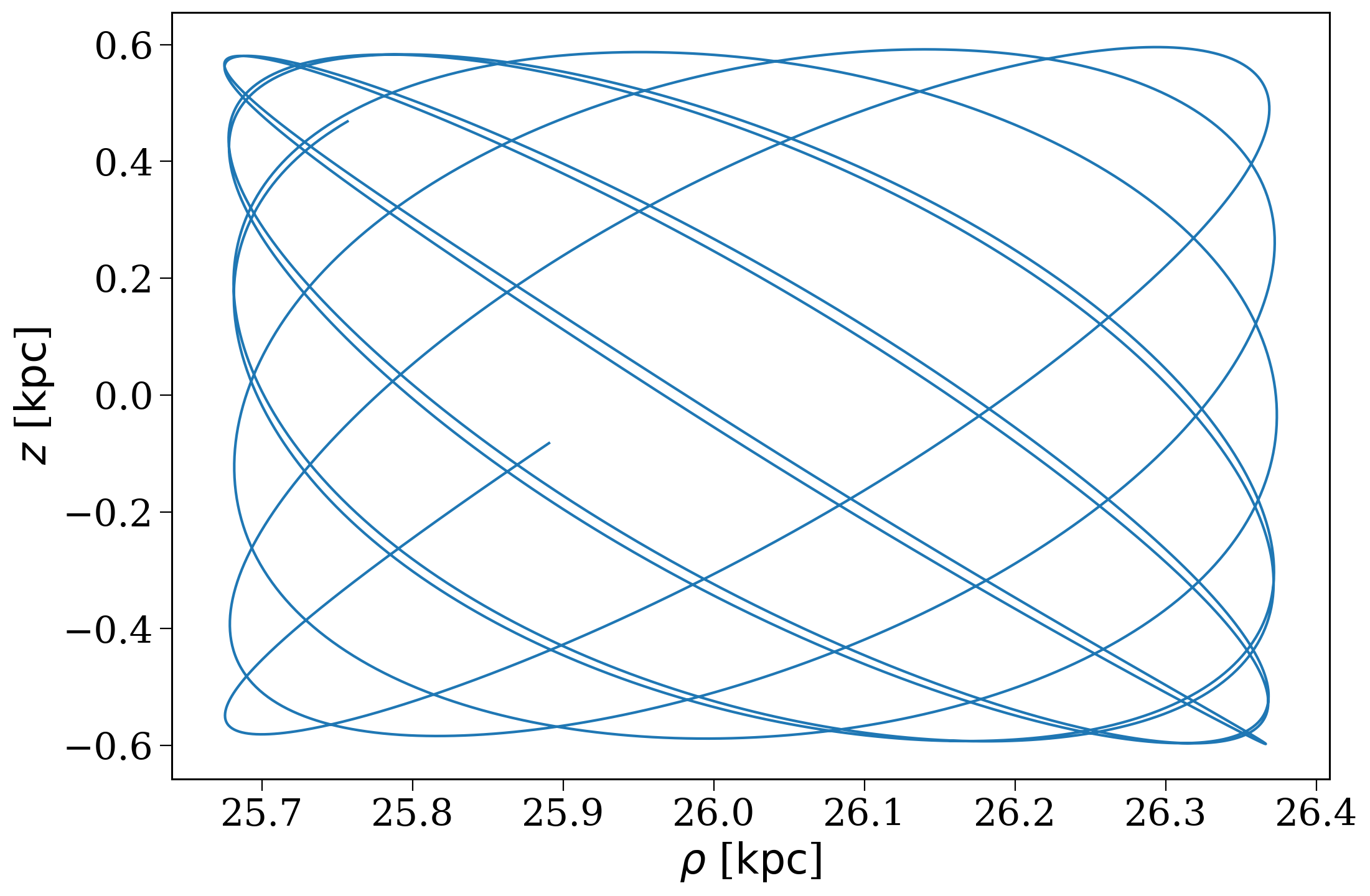
Finally, let’s bring Gala into the mix and evolve this population of binaries through a galactic potential. This will create orbits for each binary in orbits that can be accessed easily as primary_orbits and secondary_orbits.
Check out the potentials tutorial for more info and changing the galactic evolution settings (in particular the potential).
[10]:
p.perform_galactic_evolution()
p.orbits
Integrating orbits: 100%|███████████████████████████████████████████████████████████████████████████████████████████████████████████████| 1311/1311 [00:01<00:00, 669.52it/s]
[10]:
array([<Orbit cartesian, dim=3, shape=(7607,)>,
       <Orbit cartesian, dim=3, shape=(1973,)>,
       <Orbit cartesian, dim=3, shape=(1838,)>, ...,
       <Orbit cartesian, dim=3, shape=(11751,)>,
       <Orbit cartesian, dim=3, shape=(10639,)>,
       <Orbit cartesian, dim=3, shape=(8909,)>],
      shape=(1311,), dtype=object)
[11]:
fig, ax = plt.subplots()
p.orbits[np.random.randint(0, len(p.orbits))].cylindrical.plot(["rho", "z"], axes=[ax]);
The easy way#
Now that was useful to understand what’s happening behind the scenes, but for many cases you just want to efficiently create a population. This can be done all at once with the create_population().
[12]:
p.create_population()
Run for 1000 binaries
Sampled 1310 binaries
[4e-02s] Sample initial binaries
[0.3s] Evolve binaries (run COSMIC)
Integrating orbits: 100%|███████████████████████████████████████████████████████████████████████████████████████████████████████████████| 1311/1311 [00:01<00:00, 702.57it/s]
[3.0s] Integrate galactic orbits (run gala)
Overall: 3.3s
Check out the next tutorial to learn more about interpretting the outputs of these simulations.
Wrap-up#
And that’s all for this first tutorial of the basic series, nice job! We covered a lot here and much of the functionality I used will get explained in more detail in the later tutorials. Press your right arrow key for the next installment or head over to the main tutorials page for more options.
Note
This tutorial was generated from a Jupyter notebook that can be found here.