
Exploring the orbits of binaries in star clusters#
Goals and the plan#
In this case study we’re going to explore cogsworth’s ability to handle hydrodynamical zoom-in simulations and demonstrate how binary interactions can dramatically change their evolution within a cluster. In particular, let’s consider “How do supernovae in binaries change their orbits within a star cluster?”
[1]:
import cogsworth
import numpy as np
import astropy.units as u
import matplotlib.pyplot as plt
import matplotlib as mpl

from matplotlib.lines import Line2D
from matplotlib.legend_handler import HandlerLineCollection
from matplotlib.collections import LineCollection
[2]:
# this all just makes plots look nice
%config InlineBackend.figure_format = 'retina'

plt.rc('font', family='serif')
plt.rcParams['text.usetex'] = False
fs = 24

# update various fontsizes to match
params = {'figure.figsize': (12, 8),
          'legend.fontsize': fs,
          'axes.labelsize': fs,
          'xtick.labelsize': 0.9 * fs,
          'ytick.labelsize': 0.9 * fs,
          'axes.linewidth': 1.1,
          'xtick.major.size': 7,
          'xtick.minor.size': 4,
          'ytick.major.size': 7,
          'ytick.minor.size': 4}
plt.rcParams.update(params)
Prepare and process the snapshot for use#
First, we need to process a FIRE snapshot for use in our simulations. I’m going to re-use some of the code from the tutorials to prepare the \(z = 0\) snapshot from the FIRE m11h simulation. You can find this snapshot online in the FlatHub database and download it yourself!
[6]:
snap = cogsworth.hydro.utils.prepare_snapshot("../../data/snapshot_600.hdf5")
Computing the potential#
Now that the snapshot is ready to go we can work out a representation of the galactic potential. Using a self-consistent field method, one can determine the galactic potential resulting from all of the particles in the simulation. By default ``cogsworth`` constructs this potential using all of the particles in a snapshot as follows[ ]:
pot = cogsworth.hydro.potential.get_snapshot_potential(snap)
Rewinding star particles to formation#
When initialising a population from a snapshot, we want to use the *initial* state of each particle rather than its present day state (which you'll find the snapshot). Therefore you can use :func:`cogsworth.hydro.rewind.rewind_to_formation` to integrate the orbits of particles back to their starting location (using the potential we just calculated) and access their formation masses. Doing this for *every* particle would be very expensive, so we're just going to consider the particles that formed most recently.[16]:
recent_stars = snap.s[(snap.properties["time"] - snap.s["tform"]).in_units("Myr") < 150]
recent_stars
[16]:
<SimSnap "../../data/snapshot_600.hdf5::star:indexed" len=10232>
[ ]:
init_particles = cogsworth.hydro.rewind.rewind_to_formation(recent_stars, pot)
Simulate the galaxy evolution with cogsworth#
This is a big cell which would take a long time to run (hours on a laptop likely). You’re perfectly welcome to run a larger simulation like this on your own, but in our case we’re going to hone in on just one star particle to make this tractable for a laptop :D
[ ]:
# create a new HydroPopulation
p = cogsworth.hydro.pop.HydroPopulation(
    star_particles=init_particles,
    galactic_potential=pot,
    cluster_radius=3 * u.pc,
    cluster_mass=10000 * u.Msun,
    virial_parameter=1.0,
    max_ev_time=13.736521 * u.Gyr,
    processes=6,
    use_default_BSE_settings=True
)
p.create_population()
Focusing on just one star particle#
Let’s make some simple conditions to find a nice star particle. It would be nice if it was formed relatively recently (shorter orbits = faster), with a fairly low mass (fewer sampled binaries = faster) and not too close to the galactic centre (simpler orbits = faster).
Of course you might want to change these conditions to be optimised for more than just runtime!
[646]:
recent = snap.properties["time"].in_units("Gyr") - init_particles["t_form"] < 45 / 1000
but_not_too_recent = snap.properties["time"].in_units("Gyr") - init_particles["t_form"] > 40 / 1000
low_mass = init_particles["mass"] < 6000
nice_spot = ((init_particles["x"]**2 + init_particles["y"]**2)**0.5 > 5) & (abs(init_particles["z"]) < 2)
init_particles[recent & but_not_too_recent & low_mass & nice_spot].sort_values("t_form", ascending=True)
[646]:
| id | mass | Z | t_form | x | y | z | v_x | v_y | v_z | |
|---|---|---|---|---|---|---|---|---|---|---|
| 930 | 7231424 | 5768.237339 | 0.009172 | 13.692803 | 4.574098 | 2.348680 | 0.044659 | -89.862373 | 84.257595 | -24.269460 |
| 6023 | 4152982 | 5875.235044 | 0.012729 | 13.693178 | -5.368502 | -4.737183 | -0.085027 | 6.224090 | -101.217743 | 4.733644 |
| 3432 | 5859478 | 5938.063322 | 0.016559 | 13.693446 | -3.025907 | -6.940756 | 1.076242 | 78.552327 | -44.146370 | -1.410880 |
| 3434 | 1942518 | 5627.987070 | 0.013094 | 13.693581 | -3.029216 | -6.902082 | 1.078949 | 77.865572 | -44.611424 | -4.768456 |
| 6004 | 10681321 | 5724.979497 | 0.012728 | 13.693850 | -5.505565 | -4.656169 | -0.143759 | 29.948241 | -104.545041 | 6.718125 |
| 7364 | 2979855 | 5980.654508 | 0.010288 | 13.694016 | 5.941398 | 2.794227 | 0.021122 | -59.325882 | 84.707950 | 7.470200 |
| 7546 | 11912307 | 5969.536186 | 0.013675 | 13.694386 | -6.482726 | 1.239173 | -0.424132 | -43.878863 | -82.543928 | 0.267864 |
| 6702 | 7068939 | 5753.248649 | 0.005498 | 13.695323 | -4.758554 | -6.343144 | 0.271053 | 60.862610 | -84.494613 | 0.240775 |
| 201 | 10608011 | 5736.040976 | 0.012893 | 13.695389 | -5.828201 | -5.502802 | 0.474873 | 24.407445 | -117.332655 | 15.006145 |
| 7615 | 6186453 | 5991.949629 | 0.014638 | 13.695389 | -5.416391 | -4.798061 | -0.211719 | 5.015317 | -91.541480 | -1.131827 |
| 2201 | 3223458 | 5690.608873 | 0.012643 | 13.695859 | -4.626688 | -6.314460 | 0.304760 | 72.299356 | -65.095137 | 38.714513 |
| 6700 | 11805168 | 5914.844039 | 0.013854 | 13.696127 | -4.681531 | -6.376295 | 0.286601 | 60.174590 | -83.987390 | 3.842417 |
Reduce to a subset of the binaries in the star particle#
For some reason star particle 7546 speaks to me in this list so let’s run that one for all masses and timesteps of 0.5 Myr. We’re also proceed like this:
Sample the binaries
Do the stellar evolution
Pick out all of the kicked systems and a subset that don’t get kicks
Evolve those ones
This saves us running orbits for lots of binaries that don’t get kicks (whose orbits are all pretty similar anyway)
[ ]:
# create a new HydroPopulation
p = cogsworth.hydro.pop.HydroPopulation(
    star_particles=init_particles.loc[[7546]],
    galactic_potential=pot,
    cluster_radius=3 * u.pc,
    cluster_mass=10000 * u.Msun,
    virial_parameter=1.0,
    max_ev_time=13.736521 * u.Gyr,
    processes=6,
    timestep_size=0.5 * u.Myr,
    use_default_BSE_settings=True
)

# sample and evolve the binaries
p.sample_initial_binaries()
p.perform_stellar_evolution()

# extract the kicked binaries and 500 non-kicked binaries
kicked_bin_nums = p.bpp[p.bpp["evol_type"].isin([15, 16])]["bin_num"].unique()
unkicked_bin_nums = p.bin_nums[~np.isin(p.bin_nums, kicked_bin_nums)]
bin_nums = np.sort(np.concatenate([kicked_bin_nums,
                           np.random.choice(unkicked_bin_nums, 500, replace=False)]))
p = p[bin_nums]

# count binaries that ejected their secondaries with small velocities
vsys_2 = p.kick_info.loc[kicked_bin_nums]["vsys_2_total"]
small_ejections = vsys_2[(vsys_2 > 0.0) & (vsys_2 < 20.0)].index.values

# count binaries that are still bound
fbpp = p.final_bpp.loc[kicked_bin_nums]
still_bound = fbpp[(fbpp["sep"] > 0.0) & (fbpp["kstar_1"] > 10) & (fbpp["kstar_2"] > 10)]["bin_num"].values

len(kicked_bin_nums), still_bound, small_ejections
(25, array([1189]), array([ 148, 1828, 1857, 2233, 2406]))
[88]:
# evolve their orbits
p.perform_galactic_evolution()
  0%|          | 0/525 [00:00<?, ?it/s]WARNING
WARNING: AstropyDeprecationWarning: The run function is deprecated and may be removed in a future version.
        Use Integrator call method instead. [gala.potential.potential.core]: AstropyDeprecationWarning: The run function is deprecated and may be removed in a future version.
        Use Integrator call method instead. [gala.potential.potential.core]
WARNING: AstropyDeprecationWarning: The run function is deprecated and may be removed in a future version.
        Use Integrator call method instead. [gala.potential.potential.core]
WARNINGWARNING: AstropyDeprecationWarning: The run function is deprecated and may be removed in a future version.
        Use Integrator call method instead. [gala.potential.potential.core]
: AstropyDeprecationWarning: The run function is deprecated and may be removed in a future version.
        Use Integrator call method instead. [gala.potential.potential.core]WARNING
: AstropyDeprecationWarning: The run function is deprecated and may be removed in a future version.
        Use Integrator call method instead. [gala.potential.potential.core]
537it [00:15, 34.17it/s]
Create a plotting function#
Let’s make a nice function that let’s use explore the cluster for different subsets of systems.
[40]:
# YOU CAN SKIP OVER THIS CELL, IT'S ALL STYLING
# ---------------------------------------------

def add_stars(ax, starsurfacedensity=0.8, lw=1, starcolor="white", zorder=-1):
    """Don't worry too much about this function.
    It just adds a bunch of fake stars to the background of the plot (ain't it pretty)."""
    area = np.sqrt(np.sum(np.square(ax.transAxes.transform([1.,1.]) - ax.transAxes.transform([0.,0.]))))*1
    nstars = int(starsurfacedensity*area)

    #small stars
    xy = np.random.uniform(size=(nstars,2))
    ax.scatter(xy[:,0],xy[:,1], transform=ax.transAxes, alpha=0.05, s=8*lw, facecolor=starcolor, edgecolor=None, zorder=zorder, rasterized=True)
    ax.scatter(xy[:,0],xy[:,1], transform=ax.transAxes, alpha=0.1, s=4*lw, facecolor=starcolor, edgecolor=None, zorder=zorder, rasterized=True)
    ax.scatter(xy[:,0],xy[:,1], transform=ax.transAxes, alpha=0.2, s=0.5*lw, facecolor=starcolor, edgecolor=None, zorder=zorder, rasterized=True)

    #large stars
    xy = np.random.uniform(size=(nstars//4,2))
    ax.scatter(xy[:,0],xy[:,1], transform=ax.transAxes, alpha=0.1, s=15*lw, facecolor=starcolor, edgecolor=None, zorder=zorder, rasterized=True)
    ax.scatter(xy[:,0],xy[:,1], transform=ax.transAxes, alpha=0.1, s=5*lw, facecolor=starcolor, edgecolor=None, zorder=zorder, rasterized=True)
    ax.scatter(xy[:,0],xy[:,1], transform=ax.transAxes, alpha=0.5, s=2*lw, facecolor=starcolor, edgecolor=None, zorder=zorder, rasterized=True)

class HandlerColorLineCollection(HandlerLineCollection):
    """The part below this is for creating a custom legend for the plot.
    It's a bit complicated, but it's just to make the plot look nice - again don't worry."""
    def create_artists(self, legend, artist ,xdescent, ydescent,
                        width, height, fontsize,trans):
        x = np.linspace(0,width,self.get_numpoints(legend)+1)
        y = np.zeros(self.get_numpoints(legend)+1)+height/2.-ydescent
        points = np.array([x, y]).T.reshape(-1, 1, 2)
        segments = np.concatenate([points[:-1], points[1:]], axis=1)
        lc = LineCollection(segments, cmap=artist.cmap,
                            transform=trans, colors=[f'C{i}' for i in range(self.get_numpoints(legend))])
        lc.set_array(x)
        lc.set_linewidth(artist.get_linewidth())
        return [lc]
[142]:
def plot_cluster(p_osp, fig=None, ax=None,
                 extra_cluster_style={}, extra_supernova_style={}, extra_companion_style={},
                 star_kwargs={}, show=True, dark_mode=False, show_stars=False,
                 boring_limit=300, kicked_limit=7,
                 manual_kicked_bin_nums=None, verbose=False):
    """Plot a cluster of stars, showing regular binaries in one style and
    ones that experience supernovae in another.

    Parameters
    ----------
    p_osp : :class:`cogsworth.hydro.pop.HydroPopulation`
        A population containing one star particle
    fig : :class:`matplotlib.figure.Figure`, optional
        The figure to plot on, by default None
    ax : :class:`matplotlib.axes.Axes`, optional
        The axes to plot on, by default None
    extra_cluster_style : dict, optional
        Change the styling of stars that just follow the cluster, by default {}
    extra_supernova_style : dict, optional
        Change the styling of primary stars with supernovae, by default {}
    extra_companion_style : dict, optional
        Change the styling of companion stars, by default {}
    star_kwargs : dict, optional
        Parameters to pass to :func:`add_stars`, by default {}
    show : bool, optional
        Whether to show the plot, by default True
    dark_mode : bool, optional
        Whether to use a dark mode colour scheme, by default True
    show_stars : bool, optional
        Whether to show a background of fake stars, by default False
    boring_limit : int, optional
        How many boring stars (we still love them though) to show, by default 300
    kicked_limit : int, optional
        How many kicked stars (the supernovae ones) to show, by default 7
    manual_kicked_bin_nums : _type_, optional
        Use these specific binary numbers for the kicked stars instead of choosing
        a random selection (overrides `kicked_limit`), by default None

    Returns
    -------
    fig, ax : :class:`matplotlib.figure.Figure`, :class:`matplotlib.axes.Axes`
        The figure and axes that were plotted on
    """
    # create the figure if it doesn't exist
    if fig is None or ax is None:
        fig, ax = plt.subplots()

    # change the colour theme based on whether you want dark mode or not
    dark_mode_cycle = ['8dd3c7', 'feffb3', 'bfbbd9', 'fa8174', '81b1d2',
                       'fdb462', 'b3de69', 'bc82bd', 'ccebc4', 'ffed6f']
    new_cycle = ['3ed3ed', '5ab825', '5f4ecc', 'fa8174', '1f7ebf',
                 'f7972a', 'b3de69', 'bc82bd', 'ccebc4', 'ffed6f']
    plt.rcParams["axes.prop_cycle"] = mpl.cycler('color', dark_mode_cycle if dark_mode else new_cycle)

    # update the default styles
    cluster_style = {
        "color": "grey" if dark_mode else "lightgrey",
        "zorder": -1,
        "linestyle": "-",
        "alpha": 0.25,
        "autolim": True,
        "lw": 1,
        "rasterized": True
    }
    supernova_style = {
        "color": None,
        "zorder": 4,
        "linestyle": "-",
        "alpha": 0.9,
        "autolim": False,
        "lw": 2
    }
    companion_style = {
        "color": None,
        "zorder": 4,
        "linestyle": "--",
        "alpha": 0.9,
        "autolim": False,
        "lw": 2
    }
    cluster_style.update(extra_cluster_style)
    supernova_style.update(extra_supernova_style)
    companion_style.update(extra_companion_style)

    # find the kicked and unkicked binaries
    kicked_bin_nums = p_osp.bpp[p_osp.bpp["evol_type"].isin([15, 16])]["bin_num"].unique()
    unkicked_bin_nums = p_osp.bin_nums[~np.isin(p_osp.bin_nums, kicked_bin_nums)]

    # use the manual numbers if they're provided
    if manual_kicked_bin_nums is not None:
        kicked_bin_nums = manual_kicked_bin_nums
    # otherwise shuffle the kicked ones so we get a random selection
    else:
        np.random.shuffle(kicked_bin_nums)

    # these are for auto-axes limits
    x_min, x_max, y_min, y_max = np.inf, -np.inf, np.inf, -np.inf

    # track how many we've plotted
    n_boring = 0
    n_kicked = 0

    # plot unkicked ones
    for bin_num in unkicked_bin_nums:
        i = np.where(p_osp.bin_nums == bin_num)[0][0]
        if n_boring > boring_limit:
            break

        # plot them and update the axes limits
        p_osp.primary_orbits[i].cylindrical.plot(["rho", "z"], axes=ax, **cluster_style);
        x_min = min(x_min, p_osp.primary_orbits[i].cylindrical.rho.min().value)
        x_max = max(x_max, p_osp.primary_orbits[i].cylindrical.rho.max().value)
        y_min = min(y_min, p_osp.primary_orbits[i].cylindrical.z.min().value)
        y_max = max(y_max, p_osp.primary_orbits[i].cylindrical.z.max().value)
        n_boring += 1

    # plot kicked ones (without updating axes limits)
    for bin_num in kicked_bin_nums:
        i = np.where(p_osp.bin_nums == bin_num)[0][0]
        if n_kicked > kicked_limit:
            break

        # plot the primary star
        p_osp.primary_orbits[i].cylindrical.plot(["rho", "z"], axes=ax, **supernova_style);

        # if the binary was disrupted, plot the companion star after the disruption
        if p_osp.disrupted[i]:
            t_disrupt = p_osp.bpp.loc[bin_num][p_osp.bpp.loc[bin_num]["sep"] < 0]["tphys"].values[0]
            ind_disrupt = np.argwhere(p_osp.secondary_orbits[i].t
                                      - p_osp.secondary_orbits[i].t[0] < t_disrupt * u.Myr).flatten()[-1]

            companion_style["color"] = ax.lines[-1].get_color()
            p_osp.secondary_orbits[i][ind_disrupt:].cylindrical.plot(["rho", "z"], axes=ax, **companion_style);

        # add markers for each of the supernovae
        bpp_rows = p_osp.bpp.loc[bin_num]
        sn_times = []
        pre_sn_seps = []
        for evol_type, orbit in zip([15, 16], [p_osp.primary_orbits[i], p_osp.secondary_orbits[i]]):
            sn_rows = bpp_rows[bpp_rows["evol_type"] == evol_type]
            if len(sn_rows) == 0:
                continue

            t_SN = sn_rows["tphys"].values[0]
            pre_sn_seps.append(sn_rows["sep"].values[0])

            sn_times.append(t_SN)
            ind_SN = np.argwhere(orbit.t - orbit.t[0] < t_SN * u.Myr).flatten()[-1]
            ax.scatter(orbit.cylindrical.rho[ind_SN], orbit.cylindrical.z[ind_SN],
                        s=50, zorder=5, marker=(12, 2, 0), color=ax.lines[-1].get_color())


        # print some binary parameters if verbose
        if verbose:
            print(f"Binary {bin_num}")
            print(f'  Ended as {p_osp.final_bpp.loc[[bin_num]][["kstar_1", "kstar_2", "mass_1", "mass_2"]].values}, with a separation of {p_osp.final_bpp.loc[bin_num]["sep"]: 1.2f} Rsun')
            print(f'  Initial masses were {np.round(p_osp.initC.loc[[bin_num]][["mass_1", "mass_2"]].values, 2)} Msun')
            print(f'  Supernova occured at {np.round(sn_times, 2)} Myr and separation was {np.round(pre_sn_seps, 2)} Rsun')

            kick_rows = p_osp.kick_info.loc[[bin_num]]
            print(f'  Natal kick strengths were {np.round(kick_rows["natal_kick"].values, 2)} km/s, v_sys_1 was {np.round(kick_rows["vsys_1_total"].values, 2)} km/s, and v_sys_2 was {np.round(kick_rows["vsys_2_total"].values, 2)} km/s')
            print()

        n_kicked += 1

    # add the stars if requested
    if show_stars:
        add_stars(ax, starsurfacedensity=0.5, **star_kwargs)

    # update axes limits with some padding
    x_range = x_max - x_min
    y_range = y_max - y_min
    x_padding = 0.05 * x_range
    y_padding = 0.05 * y_range
    ax.set_xlim(x_min - x_padding, x_max + x_padding)
    ax.set_ylim(y_min - y_padding, y_max + y_padding)

    # add labels and legend
    ax.set_xlabel(r"Galactocentric radius, $\rho$ [kpc]")
    ax.set_ylabel(r"Galactocentric height, $z$ [kpc]")
    lc = LineCollection([[[i / 4, 0], [(i + 1) / 4, 0]] for i in range(4)], linewidths=5)
    ax.legend(handles=[lc, Line2D([0], [0], color='grey', lw=4)],
              labels=["Kicked systems", "Unkicked systems"],
              handler_map={lc: HandlerColorLineCollection(numpoints=4)},
              framealpha=0.7, loc="upper left",
              facecolor="black" if dark_mode else None,
              edgecolor="white" if dark_mode else None,
              labelcolor="white" if dark_mode else "black")

    # change background in dark mode
    if dark_mode:
        ax.set_facecolor("black")

    # show the plot if requested
    if show:
        plt.show()

    return fig, ax
Explore the data!#
Now let’s use this function to explore the simulation that we’ve run.
A random chaotic plot#
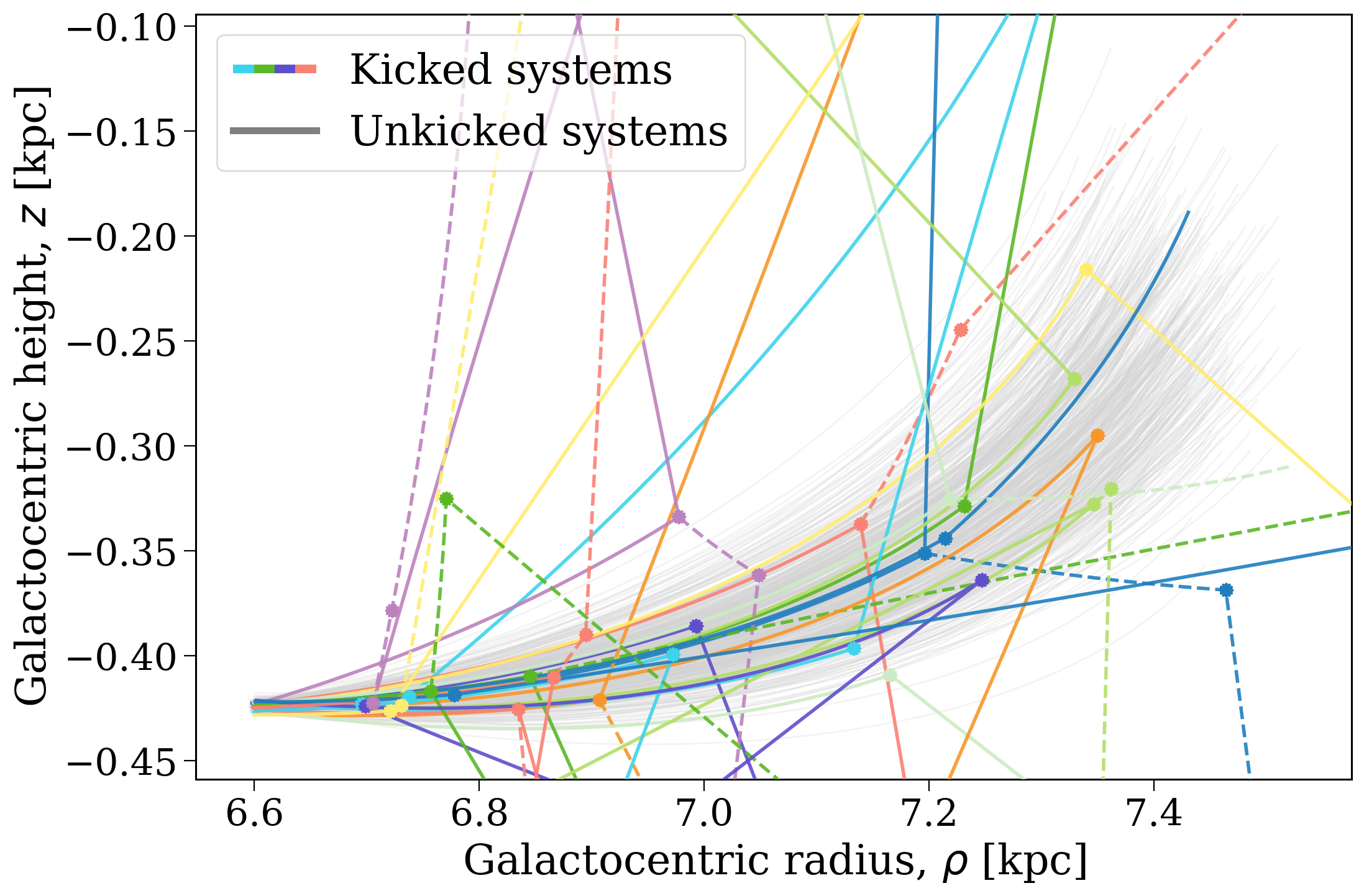
First things first let’s make a random plot. And for fun, let’s plot one with a bunch of kicked systems to really embody our inner “4 year old artist”.
[118]:
fig, ax = plot_cluster(p, kicked_limit=25, boring_limit=500)
A curated subset#
Now that’s of course a little hard to interpret, so in a case of “here’s one I made earlier”, let’s do this differently and use a couple of systems that I’ve picked out to illustrate some different scenarios.
NOTE: this cell probably won’t run for you if you are running this notebook because the exact systems that are evolved from the binary will have different bin_nums!
[202]:
fig, ax = plot_cluster(p, kicked_limit=10, boring_limit=500,
                       manual_kicked_bin_nums=[2233, 1908, 148, 1119, 1189, 552],
                       verbose=True)
Binary 2233
  Ended as [[13.         13.          1.27758353  2.21922526]], with a separation of -1.00 Rsun
  Initial masses were [[11.63  8.38]] Msun
  Supernova occured at [22.22 27.9 ] Myr and separation was [215.6  -1. ] Rsun
  Natal kick strengths were [406.34 727.73] km/s, v_sys_1 was [492.08 492.08] km/s, and v_sys_2 was [ 13.99 726.51] km/s

Binary 1908
  Ended as [[15.         13.          0.          1.26079657]], with a separation of  0.00 Rsun
  Initial masses were [[10.64  8.74]] Msun
  Supernova occured at [26.24] Myr and separation was [288.07] Rsun
  Natal kick strengths were [34.72  0.  ] km/s, v_sys_1 was [3.43 0.  ] km/s, and v_sys_2 was [0. 0.] km/s

Binary 148
  Ended as [[13.         14.          1.63037406  5.31780309]], with a separation of -1.00 Rsun
  Initial masses were [[21.48 19.9 ]] Msun
  Supernova occured at [ 9.32 11.34] Myr and separation was [309.57  -1.  ] Rsun
  Natal kick strengths were [415.1  193.39] km/s, v_sys_1 was [388.14 388.14] km/s, and v_sys_2 was [ 15.04 187.5 ] km/s

Binary 1119
  Ended as [[13.         15.          1.27758353  0.        ]], with a separation of  0.00 Rsun
  Initial masses were [[8.5  1.39]] Msun
  Supernova occured at [36.69] Myr and separation was [0.] Rsun
  Natal kick strengths were [818.61   0.  ] km/s, v_sys_1 was [818.61   0.  ] km/s, and v_sys_2 was [0. 0.] km/s

Binary 1189
  Ended as [[14.         14.         12.23541052  5.65797061]], with a separation of  54.62 Rsun
  Initial masses were [[97.9  49.93]] Msun
  Supernova occured at [3.98 5.39] Myr and separation was [3700.8   45.5] Rsun
  Natal kick strengths were [11.87 69.2 ] km/s, v_sys_1 was [ 1.25 49.52] km/s, and v_sys_2 was [0. 0.] km/s

Binary 552
  Ended as [[13.          1.          2.91306801  3.59001194]], with a separation of -1.00 Rsun
  Initial masses were [[20.92  3.57]] Msun
  Supernova occured at [9.35] Myr and separation was [36670.94] Rsun
  Natal kick strengths were [446.63   0.  ] km/s, v_sys_1 was [313.23   0.  ] km/s, and v_sys_2 was [160.16   0.  ] km/s
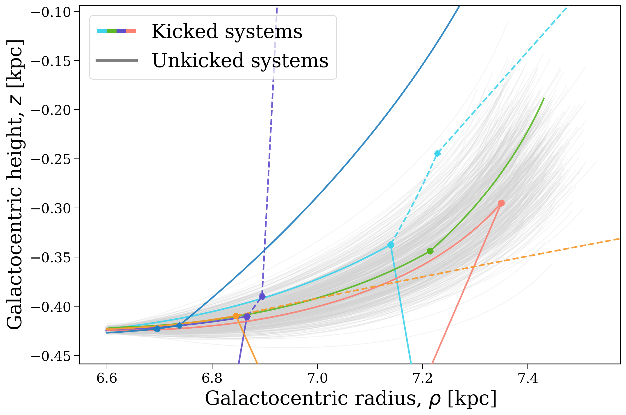
Let’s talk about the different scenarios that are occurring here:
The earliest core-collapse event occurs for the dark blue binary after \(4\, {\rm Myr}\), which is indicated by closest scatter point to the cluster origin in the lower left. This forms a \(12\, {\rm M_\odot}\) black hole and, due to a fallback fraction of \(92\%\) for the black hole, much of the explosion asymmetry is negated, resulting in a relatively weak natal kick of \(11 \, {\rm km \, s^{-1}}\), which allow1189s the binary the remain bound. The companion to this binary reaches core-collapse \(1.5\, {\rm Myr}\) later, forming a slightly less massive black hole of \(6\, {\rm M_\odot}\), with a stronger natal kick of \(70 \, {\rm km \, s^{-1}}\). Yet the binary is much tighter at this point (with a separation of \(45\, {\rm R_\odot}\)) and thus has a higher binding energy. This means that it remains bound and is ejected from the cluster as a binary black hole.
The first supernova in the orange binary occurs \(9\, {\rm Myr}\) after the cluster birth and forms a neutron star with a natal kick of \(447 \, {\rm km \, s^{-1}}\). This kick disrupts the binary orbit, such that both stars are ejected from the cluster. The secondary is a lower mass star of \(3.6\, {\rm M_\odot}\) and so experiences no supernova, but it is ejected from the cluster at \(160 \, {\rm km \, s^{-1}}\) and as such is now a runaway star.
The purple binary experiences its first supernova at \(9.3\, {\rm Myr}\) and, similar to the orange binary, this forms a \(1.6\, {\rm M_\odot}\) NS with a natal kick of \(415 \, {\rm km \, s^{-1}}\) that unbinds the binary. Interestingly, the mass ratio of this system is inverted, such that the companion forms a more massive \(5.3\, {\rm M_\odot}\) black hole after its core-collapse \(2\, {\rm Myr}\) later. This inversion occurred as a result of significant, near conservative mass transfer from the primary star during its Hertzsprung gap phase \(1.2\, {\rm Myr}\) before it reached core-collapse.
Both supernovae for the light blue binary form neutron stars (of \(1.3\) and \(2.2\, {\rm M_\odot}\) respectively) with strong kicks (of \(406\) and \(728 \, {\rm km \, s^{-1}}\) respectively), which disrupt the binary and eject both neutron stars rapidly from the cluster.
The primary star in the green binary reaches core-collapse \(26\, {\rm Myr}\) after the cluster birth, forming a neutron star of \(1.27\, {\rm M_\odot}\). The star explodes as an electron-capture supernova and thus its kick is assumed to be weaker, in this case the drawn natal kick is only \(35 \, {\rm km \, s^{-1}}\) and the binary remains bound. In addition, as a result of the angle of the kick relative to the binary’s orbit, this only results in a \(3.4 \, {\rm km \, s^{-1}}\) change to the systemic velocity of the binary. As a result, the binary remains bound to the cluster for its subsequent evolution.
Finally, after \({\sim}33\, {\rm Myr}\), the primary star in the red binary finishes its main sequence, As it expands during its Hertzsprung gap phase, it overflows its Roche lobe, causing unstable mass transfer which leads to a merger. The merged star then reaches supernova \(4\, {\rm Myr}\) later, forming a neutron star which is ejected by its strong natal kick of \(819 \, {\rm km \, s^{-1}}\), in almost the opposite direction to the cluster’s centre of mass motion.
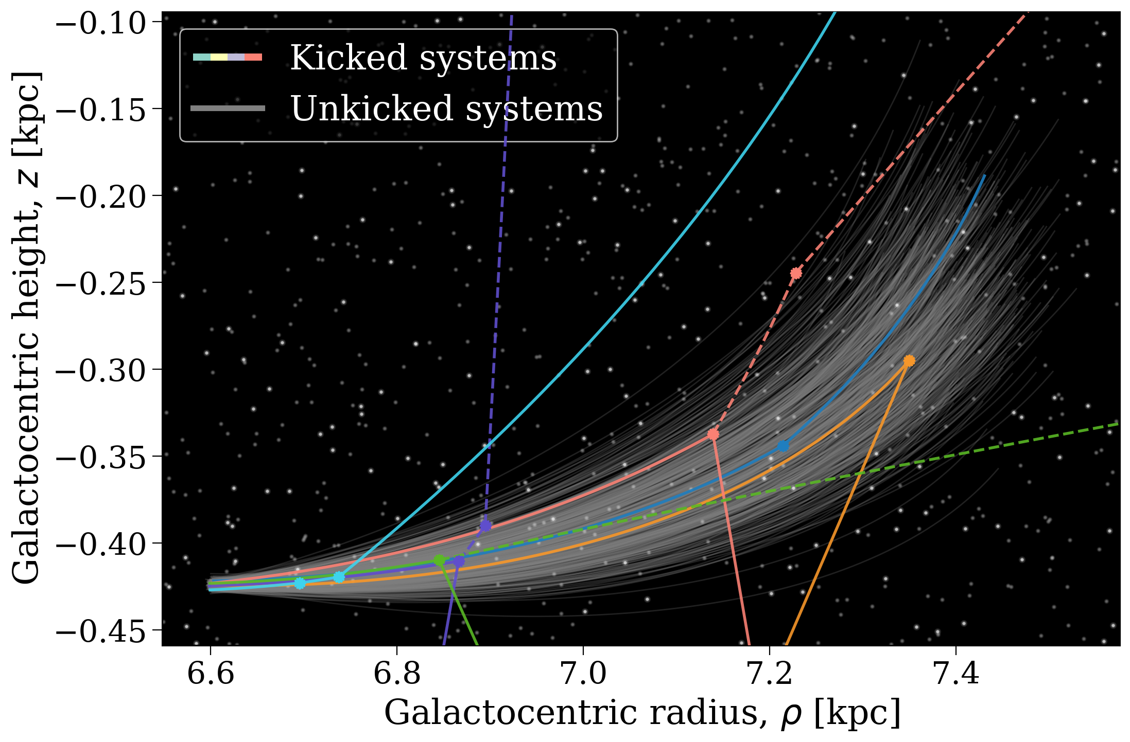
A pretty version#
And finally, just for fun, we can make a version of the plot in dark mode that has some fake stars in the background :star:
[124]:
fig, ax = plot_cluster(p, dark_mode=True, show_stars=True, kicked_limit=50, boring_limit=500,
                       manual_kicked_bin_nums=[1189, 552, 148, 2233, 1908, 1119])
Note
This tutorial was generated from a Jupyter notebook that can be found here.