
Understanding the simulation outputs#
Now that you’ve run your first cogsworth simulation it’s time to understand how to interpret the outputs!
Learning Goals#
By the end of this tutorial you should know how to:
Retrieve initial conditions from
initCandinitial_galaxyInterpret stellar evolution information from the
bpp,bcmandkick_infotablesUnderstand how to access orbits of systems as well as final positions and velocities with
orbits,final_posandfinal_vel
[1]:
import cogsworth
import numpy as np
import astropy.units as u
import matplotlib.pyplot as plt
import pandas as pd
[2]:
# this all just makes plots look nice
%config InlineBackend.figure_format = 'retina'

plt.rc('font', family='serif')
plt.rcParams['text.usetex'] = False
fs = 24

# update various fontsizes to match
params = {'figure.figsize': (12, 8),
          'legend.fontsize': fs,
          'axes.labelsize': fs,
          'xtick.labelsize': 0.9 * fs,
          'ytick.labelsize': 0.9 * fs,
          'axes.linewidth': 1.1,
          'xtick.major.size': 7,
          'xtick.minor.size': 4,
          'ytick.major.size': 7,
          'ytick.minor.size': 4}
plt.rcParams.update(params)
pd.options.display.max_columns = 999
Let’s quickly recreate a similar population to the one in the last tutorial, but now biasing towards systems likely to create neutron stars and black holes (so that the later parts of this tutorial are more interesting 😉)
[3]:
p = cogsworth.pop.Population(100, final_kstar1=[13, 14], final_kstar2=[13, 14],
                             use_default_BSE_settings=True)
p.create_population()
Run for 100 binaries
Sampled 100 binaries
[1e-02s] Sample initial binaries
[0.2s] Evolve binaries (run COSMIC)
Integrating orbits: 100%|██████████| 119/119 [00:00<00:00, 1161.67it/s]
[0.5s] Integrate galactic orbits (run gala)
Overall: 0.7s
Initial conditions#
Though not technically and output of your simulation, the sampled initial population is useful to access for reproducibility. The initC table describes the initial conditions for the stellar evolution of every system, whilst the initial_galaxy gives the position, velocity, time and metallicity at which the system is born.
initial_binaries - Stellar initial conditions#
The initial_binaries table is an output of COSMIC and is a Pandas DataFrame with a row for each sampled system. The columns describe the binary initial conditions (e.g. initial masses) as well as stellar evolution settings (e.g. common-envelope alpha).
[4]:
p.initial_binaries
[4]:
| kstar_1 | kstar_2 | mass_1 | mass_2 | porb | ecc | metallicity | binfrac | tphysf | mass0_1 | mass0_2 | rad_1 | rad_2 | lum_1 | lum_2 | massc_1 | massc_2 | radc_1 | radc_2 | menv_1 | menv_2 | renv_1 | renv_2 | omega_spin_1 | omega_spin_2 | B_1 | B_2 | bacc_1 | bacc_2 | tacc_1 | tacc_2 | epoch_1 | epoch_2 | tms_1 | tms_2 | bhspin_1 | bhspin_2 | tphys | neta | bwind | hewind | alpha1 | lambdaf | ceflag | tflag | ifflag | wdflag | pisn | ppi_co_shift | ppi_extra_ml | rtmsflag | bhflag | remnantflag | fryer_mass_limit | maltsev_mode | maltsev_fallback | maltsev_pf_prob | grflag | bhms_coll_flag | wd_mass_lim | cekickflag | cemergeflag | cehestarflag | mxns | pts1 | pts2 | pts3 | ecsn | ecsn_mlow | aic | ussn | sigma | sigmadiv | bhsigmafrac | polar_kick_angle | mm_mu_ns | mm_mu_bh | beta | xi | acc2 | epsnov | eddfac | gamma | don_lim | acc_lim | bdecayfac | bconst | ck | windflag | qcflag | eddlimflag | LBV_flag | dtp | randomseed | bhspinflag | bhspinmag | rejuv_fac | rejuvflag | htpmb | ST_cr | ST_tide | rembar_massloss | zsun | kickflag | bin_num | natal_kick_1 | phi_1 | theta_1 | mean_anomaly_1 | randomseed_1 | natal_kick_2 | phi_2 | theta_2 | mean_anomaly_2 | randomseed_2 | qcrit_0 | qcrit_1 | qcrit_2 | qcrit_3 | qcrit_4 | qcrit_5 | qcrit_6 | qcrit_7 | qcrit_8 | qcrit_9 | qcrit_10 | qcrit_11 | qcrit_12 | qcrit_13 | qcrit_14 | qcrit_15 | fprimc_0 | fprimc_1 | fprimc_2 | fprimc_3 | fprimc_4 | fprimc_5 | fprimc_6 | fprimc_7 | fprimc_8 | fprimc_9 | fprimc_10 | fprimc_11 | fprimc_12 | fprimc_13 | fprimc_14 | fprimc_15 | phase_sn_1 | phase_sn_2 | inc_sn_1 | inc_sn_2 | |
|---|---|---|---|---|---|---|---|---|---|---|---|---|---|---|---|---|---|---|---|---|---|---|---|---|---|---|---|---|---|---|---|---|---|---|---|---|---|---|---|---|---|---|---|---|---|---|---|---|---|---|---|---|---|---|---|---|---|---|---|---|---|---|---|---|---|---|---|---|---|---|---|---|---|---|---|---|---|---|---|---|---|---|---|---|---|---|---|---|---|---|---|---|---|---|---|---|---|---|---|---|---|---|---|---|---|---|---|---|---|---|---|---|---|---|---|---|---|---|---|---|---|---|---|---|---|---|---|---|---|---|---|---|---|---|---|---|---|---|---|---|---|---|---|---|---|---|---|---|---|---|---|
| 0 | 1.0 | 1.0 | 4.698050 | 3.797264 | 17.174898 | 0.242255 | 0.030000 | 1.0 | 2827.301106 | 4.698050 | 3.797264 | 0.0 | 0.0 | 0.0 | 0.0 | 0.0 | 0.0 | 0.0 | 0.0 | 0.0 | 0.0 | 0.0 | 0.0 | 0.0 | 0.0 | 0.0 | 0.0 | 0.0 | 0.0 | 0.0 | 0.0 | 0.0 | 0.0 | 0.0 | 0.0 | 0.0 | 0.0 | 0.0 | 0.5 | 0.0 | 0.5 | 1.0 | 0.0 | 1 | 1 | 1 | 1 | -2 | 0.0 | 0.0 | 0 | 1 | 4 | 0 | 0 | 0.5 | 0.1 | 1 | 0 | 1 | 2 | 1 | 0 | 3.0 | 0.0010 | 0.010 | 0.020 | 2.25 | 1.6 | 1 | 1 | 265.0 | -20.0 | 1.0 | 90.0 | 400.0 | 200.0 | 0.125 | 0.5 | 1.5 | 0.001 | 10 | -2 | -1 | -1 | 1 | 3000 | 1000 | 3 | 5 | 0 | 1 | 2827.301106 | 794680645 | 0 | 0.0 | 1.0 | 0 | 1 | 1 | 1 | 0.5 | 0.014 | 5 | 0 | -100.000000 | -100.000000 | -100.000000 | -100.000000 | 0.0 | -100.000000 | -100.000000 | -100.000000 | -100.0 | 0.000000e+00 | 0.0 | 0.0 | 0.0 | 0.0 | 0.0 | 0.0 | 0.0 | 0.0 | 0.0 | 0.0 | 0.0 | 0.0 | 0.0 | 0.0 | 0.0 | 0.0 | 0.095238 | 0.095238 | 0.095238 | 0.095238 | 0.095238 | 0.095238 | 0.095238 | 0.095238 | 0.095238 | 0.095238 | 0.095238 | 0.095238 | 0.095238 | 0.095238 | 0.095238 | 0.095238 | 3.744726 | 4.083493 | 1.362724 | 0.725437 |
| 1 | 1.0 | 1.0 | 7.325796 | 3.959182 | 659.303111 | 0.145843 | 0.017036 | 1.0 | 7906.223993 | 7.325796 | 3.959182 | 0.0 | 0.0 | 0.0 | 0.0 | 0.0 | 0.0 | 0.0 | 0.0 | 0.0 | 0.0 | 0.0 | 0.0 | 0.0 | 0.0 | 0.0 | 0.0 | 0.0 | 0.0 | 0.0 | 0.0 | 0.0 | 0.0 | 0.0 | 0.0 | 0.0 | 0.0 | 0.0 | 0.5 | 0.0 | 0.5 | 1.0 | 0.0 | 1 | 1 | 1 | 1 | -2 | 0.0 | 0.0 | 0 | 1 | 4 | 0 | 0 | 0.5 | 0.1 | 1 | 0 | 1 | 2 | 1 | 0 | 3.0 | 0.0010 | 0.010 | 0.020 | 2.25 | 1.6 | 1 | 1 | 265.0 | -20.0 | 1.0 | 90.0 | 400.0 | 200.0 | 0.125 | 0.5 | 1.5 | 0.001 | 10 | -2 | -1 | -1 | 1 | 3000 | 1000 | 3 | 5 | 0 | 1 | 7906.223993 | 462462847 | 0 | 0.0 | 1.0 | 0 | 1 | 1 | 1 | 0.5 | 0.014 | 5 | 1 | -100.000000 | -100.000000 | -100.000000 | -100.000000 | 0.0 | -100.000000 | -100.000000 | -100.000000 | -100.0 | 0.000000e+00 | 0.0 | 0.0 | 0.0 | 0.0 | 0.0 | 0.0 | 0.0 | 0.0 | 0.0 | 0.0 | 0.0 | 0.0 | 0.0 | 0.0 | 0.0 | 0.0 | 0.095238 | 0.095238 | 0.095238 | 0.095238 | 0.095238 | 0.095238 | 0.095238 | 0.095238 | 0.095238 | 0.095238 | 0.095238 | 0.095238 | 0.095238 | 0.095238 | 0.095238 | 0.095238 | 1.822689 | 3.783131 | 1.307289 | 1.399754 |
| 2 | 1.0 | 1.0 | 22.209909 | 18.066209 | 2.017690 | 0.001033 | 0.011458 | 1.0 | 5318.706038 | 22.209909 | 18.066209 | 0.0 | 0.0 | 0.0 | 0.0 | 0.0 | 0.0 | 0.0 | 0.0 | 0.0 | 0.0 | 0.0 | 0.0 | 0.0 | 0.0 | 0.0 | 0.0 | 0.0 | 0.0 | 0.0 | 0.0 | 0.0 | 0.0 | 0.0 | 0.0 | 0.0 | 0.0 | 0.0 | 0.5 | 0.0 | 0.5 | 1.0 | 0.0 | 1 | 1 | 1 | 1 | -2 | 0.0 | 0.0 | 0 | 1 | 4 | 0 | 0 | 0.5 | 0.1 | 1 | 0 | 1 | 2 | 1 | 0 | 3.0 | 0.0010 | 0.010 | 0.020 | 2.25 | 1.6 | 1 | 1 | 265.0 | -20.0 | 1.0 | 90.0 | 400.0 | 200.0 | 0.125 | 0.5 | 1.5 | 0.001 | 10 | -2 | -1 | -1 | 1 | 3000 | 1000 | 3 | 5 | 0 | 1 | 5318.706038 | -514529300 | 0 | 0.0 | 1.0 | 0 | 1 | 1 | 1 | 0.5 | 0.014 | 5 | 2 | 97.322127 | -24.636763 | 124.831960 | -100.000000 | -514529300.0 | -100.000000 | -100.000000 | -100.000000 | -100.0 | 0.000000e+00 | 0.0 | 0.0 | 0.0 | 0.0 | 0.0 | 0.0 | 0.0 | 0.0 | 0.0 | 0.0 | 0.0 | 0.0 | 0.0 | 0.0 | 0.0 | 0.0 | 0.095238 | 0.095238 | 0.095238 | 0.095238 | 0.095238 | 0.095238 | 0.095238 | 0.095238 | 0.095238 | 0.095238 | 0.095238 | 0.095238 | 0.095238 | 0.095238 | 0.095238 | 0.095238 | 0.247182 | 4.918894 | 0.290235 | 2.632831 |
| 3 | 1.0 | 1.0 | 51.585165 | 27.155132 | 4401.558908 | 0.271034 | 0.006022 | 1.0 | 7705.250269 | 51.585165 | 27.155132 | 0.0 | 0.0 | 0.0 | 0.0 | 0.0 | 0.0 | 0.0 | 0.0 | 0.0 | 0.0 | 0.0 | 0.0 | 0.0 | 0.0 | 0.0 | 0.0 | 0.0 | 0.0 | 0.0 | 0.0 | 0.0 | 0.0 | 0.0 | 0.0 | 0.0 | 0.0 | 0.0 | 0.5 | 0.0 | 0.5 | 1.0 | 0.0 | 1 | 1 | 1 | 1 | -2 | 0.0 | 0.0 | 0 | 1 | 4 | 0 | 0 | 0.5 | 0.1 | 1 | 0 | 1 | 2 | 1 | 0 | 3.0 | 0.0003 | 0.003 | 0.006 | 2.25 | 1.6 | 1 | 1 | 265.0 | -20.0 | 1.0 | 90.0 | 400.0 | 200.0 | 0.125 | 0.5 | 1.5 | 0.001 | 10 | -2 | -1 | -1 | 1 | 3000 | 1000 | 3 | 5 | 0 | 1 | 7705.250269 | 954140660 | 0 | 0.0 | 1.0 | 0 | 1 | 1 | 1 | 0.5 | 0.014 | 5 | 3 | 63.416925 | 6.800539 | 106.803696 | 333.993301 | -954140660.0 | 179.721303 | 40.915287 | 292.643380 | -100.0 | 7.436287e+08 | 0.0 | 0.0 | 0.0 | 0.0 | 0.0 | 0.0 | 0.0 | 0.0 | 0.0 | 0.0 | 0.0 | 0.0 | 0.0 | 0.0 | 0.0 | 0.0 | 0.095238 | 0.095238 | 0.095238 | 0.095238 | 0.095238 | 0.095238 | 0.095238 | 0.095238 | 0.095238 | 0.095238 | 0.095238 | 0.095238 | 0.095238 | 0.095238 | 0.095238 | 0.095238 | 3.893668 | 2.813141 | 1.258837 | 1.607091 |
| 4 | 1.0 | 1.0 | 3.951983 | 3.003154 | 72425.309853 | 0.699177 | 0.014759 | 1.0 | 731.789346 | 3.951983 | 3.003154 | 0.0 | 0.0 | 0.0 | 0.0 | 0.0 | 0.0 | 0.0 | 0.0 | 0.0 | 0.0 | 0.0 | 0.0 | 0.0 | 0.0 | 0.0 | 0.0 | 0.0 | 0.0 | 0.0 | 0.0 | 0.0 | 0.0 | 0.0 | 0.0 | 0.0 | 0.0 | 0.0 | 0.5 | 0.0 | 0.5 | 1.0 | 0.0 | 1 | 1 | 1 | 1 | -2 | 0.0 | 0.0 | 0 | 1 | 4 | 0 | 0 | 0.5 | 0.1 | 1 | 0 | 1 | 2 | 1 | 0 | 3.0 | 0.0010 | 0.010 | 0.020 | 2.25 | 1.6 | 1 | 1 | 265.0 | -20.0 | 1.0 | 90.0 | 400.0 | 200.0 | 0.125 | 0.5 | 1.5 | 0.001 | 10 | -2 | -1 | -1 | 1 | 3000 | 1000 | 3 | 5 | 0 | 1 | 731.789346 | -1082638121 | 0 | 0.0 | 1.0 | 0 | 1 | 1 | 1 | 0.5 | 0.014 | 5 | 4 | -100.000000 | -100.000000 | -100.000000 | -100.000000 | 0.0 | -100.000000 | -100.000000 | -100.000000 | -100.0 | 0.000000e+00 | 0.0 | 0.0 | 0.0 | 0.0 | 0.0 | 0.0 | 0.0 | 0.0 | 0.0 | 0.0 | 0.0 | 0.0 | 0.0 | 0.0 | 0.0 | 0.0 | 0.095238 | 0.095238 | 0.095238 | 0.095238 | 0.095238 | 0.095238 | 0.095238 | 0.095238 | 0.095238 | 0.095238 | 0.095238 | 0.095238 | 0.095238 | 0.095238 | 0.095238 | 0.095238 | 4.403690 | 5.358024 | 0.702274 | 1.622489 |
| ... | ... | ... | ... | ... | ... | ... | ... | ... | ... | ... | ... | ... | ... | ... | ... | ... | ... | ... | ... | ... | ... | ... | ... | ... | ... | ... | ... | ... | ... | ... | ... | ... | ... | ... | ... | ... | ... | ... | ... | ... | ... | ... | ... | ... | ... | ... | ... | ... | ... | ... | ... | ... | ... | ... | ... | ... | ... | ... | ... | ... | ... | ... | ... | ... | ... | ... | ... | ... | ... | ... | ... | ... | ... | ... | ... | ... | ... | ... | ... | ... | ... | ... | ... | ... | ... | ... | ... | ... | ... | ... | ... | ... | ... | ... | ... | ... | ... | ... | ... | ... | ... | ... | ... | ... | ... | ... | ... | ... | ... | ... | ... | ... | ... | ... | ... | ... | ... | ... | ... | ... | ... | ... | ... | ... | ... | ... | ... | ... | ... | ... | ... | ... | ... | ... | ... | ... | ... | ... | ... | ... | ... | ... | ... | ... | ... | ... | ... | ... | ... | ... | ... |
| 95 | 1.0 | 1.0 | 4.174748 | 3.022807 | 1.652611 | 0.067768 | 0.008243 | 1.0 | 8381.976082 | 4.174748 | 3.022807 | 0.0 | 0.0 | 0.0 | 0.0 | 0.0 | 0.0 | 0.0 | 0.0 | 0.0 | 0.0 | 0.0 | 0.0 | 0.0 | 0.0 | 0.0 | 0.0 | 0.0 | 0.0 | 0.0 | 0.0 | 0.0 | 0.0 | 0.0 | 0.0 | 0.0 | 0.0 | 0.0 | 0.5 | 0.0 | 0.5 | 1.0 | 0.0 | 1 | 1 | 1 | 1 | -2 | 0.0 | 0.0 | 0 | 1 | 4 | 0 | 0 | 0.5 | 0.1 | 1 | 0 | 1 | 2 | 1 | 0 | 3.0 | 0.0010 | 0.010 | 0.020 | 2.25 | 1.6 | 1 | 1 | 265.0 | -20.0 | 1.0 | 90.0 | 400.0 | 200.0 | 0.125 | 0.5 | 1.5 | 0.001 | 10 | -2 | -1 | -1 | 1 | 3000 | 1000 | 3 | 5 | 0 | 1 | 8381.976082 | -823025274 | 0 | 0.0 | 1.0 | 0 | 1 | 1 | 1 | 0.5 | 0.014 | 5 | 95 | -100.000000 | -100.000000 | -100.000000 | -100.000000 | 0.0 | -100.000000 | -100.000000 | -100.000000 | -100.0 | 0.000000e+00 | 0.0 | 0.0 | 0.0 | 0.0 | 0.0 | 0.0 | 0.0 | 0.0 | 0.0 | 0.0 | 0.0 | 0.0 | 0.0 | 0.0 | 0.0 | 0.0 | 0.095238 | 0.095238 | 0.095238 | 0.095238 | 0.095238 | 0.095238 | 0.095238 | 0.095238 | 0.095238 | 0.095238 | 0.095238 | 0.095238 | 0.095238 | 0.095238 | 0.095238 | 0.095238 | 0.472626 | 3.362548 | 2.240190 | 1.218247 |
| 96 | 1.0 | 1.0 | 7.136089 | 5.705648 | 3547.431919 | 0.220289 | 0.014787 | 1.0 | 7935.521312 | 7.136089 | 5.705648 | 0.0 | 0.0 | 0.0 | 0.0 | 0.0 | 0.0 | 0.0 | 0.0 | 0.0 | 0.0 | 0.0 | 0.0 | 0.0 | 0.0 | 0.0 | 0.0 | 0.0 | 0.0 | 0.0 | 0.0 | 0.0 | 0.0 | 0.0 | 0.0 | 0.0 | 0.0 | 0.0 | 0.5 | 0.0 | 0.5 | 1.0 | 0.0 | 1 | 1 | 1 | 1 | -2 | 0.0 | 0.0 | 0 | 1 | 4 | 0 | 0 | 0.5 | 0.1 | 1 | 0 | 1 | 2 | 1 | 0 | 3.0 | 0.0010 | 0.010 | 0.020 | 2.25 | 1.6 | 1 | 1 | 265.0 | -20.0 | 1.0 | 90.0 | 400.0 | 200.0 | 0.125 | 0.5 | 1.5 | 0.001 | 10 | -2 | -1 | -1 | 1 | 3000 | 1000 | 3 | 5 | 0 | 1 | 7935.521312 | 1670782002 | 0 | 0.0 | 1.0 | 0 | 1 | 1 | 1 | 0.5 | 0.014 | 5 | 96 | -100.000000 | -100.000000 | -100.000000 | -100.000000 | 0.0 | -100.000000 | -100.000000 | -100.000000 | -100.0 | 0.000000e+00 | 0.0 | 0.0 | 0.0 | 0.0 | 0.0 | 0.0 | 0.0 | 0.0 | 0.0 | 0.0 | 0.0 | 0.0 | 0.0 | 0.0 | 0.0 | 0.0 | 0.095238 | 0.095238 | 0.095238 | 0.095238 | 0.095238 | 0.095238 | 0.095238 | 0.095238 | 0.095238 | 0.095238 | 0.095238 | 0.095238 | 0.095238 | 0.095238 | 0.095238 | 0.095238 | 2.722685 | 4.844767 | 1.654927 | 1.298071 |
| 97 | 1.0 | 1.0 | 8.632751 | 8.593908 | 4.382319 | 0.022096 | 0.015533 | 1.0 | 8405.868131 | 8.632751 | 8.593908 | 0.0 | 0.0 | 0.0 | 0.0 | 0.0 | 0.0 | 0.0 | 0.0 | 0.0 | 0.0 | 0.0 | 0.0 | 0.0 | 0.0 | 0.0 | 0.0 | 0.0 | 0.0 | 0.0 | 0.0 | 0.0 | 0.0 | 0.0 | 0.0 | 0.0 | 0.0 | 0.0 | 0.5 | 0.0 | 0.5 | 1.0 | 0.0 | 1 | 1 | 1 | 1 | -2 | 0.0 | 0.0 | 0 | 1 | 4 | 0 | 0 | 0.5 | 0.1 | 1 | 0 | 1 | 2 | 1 | 0 | 3.0 | 0.0010 | 0.010 | 0.020 | 2.25 | 1.6 | 1 | 1 | 265.0 | -20.0 | 1.0 | 90.0 | 400.0 | 200.0 | 0.125 | 0.5 | 1.5 | 0.001 | 10 | -2 | -1 | -1 | 1 | 3000 | 1000 | 3 | 5 | 0 | 1 | 8405.868131 | -713627973 | 0 | 0.0 | 1.0 | 0 | 1 | 1 | 1 | 0.5 | 0.014 | 5 | 97 | 148.660836 | -6.575601 | 348.208601 | -100.000000 | -713627973.0 | -100.000000 | -100.000000 | -100.000000 | -100.0 | 0.000000e+00 | 0.0 | 0.0 | 0.0 | 0.0 | 0.0 | 0.0 | 0.0 | 0.0 | 0.0 | 0.0 | 0.0 | 0.0 | 0.0 | 0.0 | 0.0 | 0.0 | 0.095238 | 0.095238 | 0.095238 | 0.095238 | 0.095238 | 0.095238 | 0.095238 | 0.095238 | 0.095238 | 0.095238 | 0.095238 | 0.095238 | 0.095238 | 0.095238 | 0.095238 | 0.095238 | 5.424119 | 2.382820 | 2.050053 | 1.775458 |
| 98 | 1.0 | 1.0 | 49.700884 | 37.604461 | 2334.535495 | 0.009498 | 0.018127 | 1.0 | 8614.507070 | 49.700884 | 37.604461 | 0.0 | 0.0 | 0.0 | 0.0 | 0.0 | 0.0 | 0.0 | 0.0 | 0.0 | 0.0 | 0.0 | 0.0 | 0.0 | 0.0 | 0.0 | 0.0 | 0.0 | 0.0 | 0.0 | 0.0 | 0.0 | 0.0 | 0.0 | 0.0 | 0.0 | 0.0 | 0.0 | 0.5 | 0.0 | 0.5 | 1.0 | 0.0 | 1 | 1 | 1 | 1 | -2 | 0.0 | 0.0 | 0 | 1 | 4 | 0 | 0 | 0.5 | 0.1 | 1 | 0 | 1 | 2 | 1 | 0 | 3.0 | 0.0003 | 0.003 | 0.006 | 2.25 | 1.6 | 1 | 1 | 265.0 | -20.0 | 1.0 | 90.0 | 400.0 | 200.0 | 0.125 | 0.5 | 1.5 | 0.001 | 10 | -2 | -1 | -1 | 1 | 3000 | 1000 | 3 | 5 | 0 | 1 | 8614.507070 | -619207706 | 0 | 0.0 | 1.0 | 0 | 1 | 1 | 1 | 0.5 | 0.014 | 5 | 98 | 126.484524 | 12.444072 | 28.004209 | 308.889477 | -619207706.0 | 93.645108 | -5.015615 | 334.551909 | -100.0 | 2.051889e+09 | 0.0 | 0.0 | 0.0 | 0.0 | 0.0 | 0.0 | 0.0 | 0.0 | 0.0 | 0.0 | 0.0 | 0.0 | 0.0 | 0.0 | 0.0 | 0.0 | 0.095238 | 0.095238 | 0.095238 | 0.095238 | 0.095238 | 0.095238 | 0.095238 | 0.095238 | 0.095238 | 0.095238 | 0.095238 | 0.095238 | 0.095238 | 0.095238 | 0.095238 | 0.095238 | 1.656223 | 4.543093 | 0.081508 | 1.153337 |
| 99 | 1.0 | 1.0 | 15.961007 | 13.816449 | 52.937913 | 0.004498 | 0.005887 | 1.0 | 8719.861062 | 15.961007 | 13.816449 | 0.0 | 0.0 | 0.0 | 0.0 | 0.0 | 0.0 | 0.0 | 0.0 | 0.0 | 0.0 | 0.0 | 0.0 | 0.0 | 0.0 | 0.0 | 0.0 | 0.0 | 0.0 | 0.0 | 0.0 | 0.0 | 0.0 | 0.0 | 0.0 | 0.0 | 0.0 | 0.0 | 0.5 | 0.0 | 0.5 | 1.0 | 0.0 | 1 | 1 | 1 | 1 | -2 | 0.0 | 0.0 | 0 | 1 | 4 | 0 | 0 | 0.5 | 0.1 | 1 | 0 | 1 | 2 | 1 | 0 | 3.0 | 0.0010 | 0.010 | 0.020 | 2.25 | 1.6 | 1 | 1 | 265.0 | -20.0 | 1.0 | 90.0 | 400.0 | 200.0 | 0.125 | 0.5 | 1.5 | 0.001 | 10 | -2 | -1 | -1 | 1 | 3000 | 1000 | 3 | 5 | 0 | 1 | 8719.861062 | 893556274 | 0 | 0.0 | 1.0 | 0 | 1 | 1 | 1 | 0.5 | 0.014 | 5 | 99 | 1172.966666 | 32.163143 | 21.069551 | -100.000000 | -893556274.0 | -100.000000 | -100.000000 | -100.000000 | -100.0 | 0.000000e+00 | 0.0 | 0.0 | 0.0 | 0.0 | 0.0 | 0.0 | 0.0 | 0.0 | 0.0 | 0.0 | 0.0 | 0.0 | 0.0 | 0.0 | 0.0 | 0.0 | 0.095238 | 0.095238 | 0.095238 | 0.095238 | 0.095238 | 0.095238 | 0.095238 | 0.095238 | 0.095238 | 0.095238 | 0.095238 | 0.095238 | 0.095238 | 0.095238 | 0.095238 | 0.095238 | 4.526432 | 4.432509 | 0.580866 | 0.933846 |
100 rows × 151 columns
You could use this table to access only binaries that particular initial conditions, e.g. taking only those with eccentric initial orbits
[5]:
p.initial_binaries[p.initial_binaries["ecc"] > 0.8]
[5]:
| kstar_1 | kstar_2 | mass_1 | mass_2 | porb | ecc | metallicity | binfrac | tphysf | mass0_1 | mass0_2 | rad_1 | rad_2 | lum_1 | lum_2 | massc_1 | massc_2 | radc_1 | radc_2 | menv_1 | menv_2 | renv_1 | renv_2 | omega_spin_1 | omega_spin_2 | B_1 | B_2 | bacc_1 | bacc_2 | tacc_1 | tacc_2 | epoch_1 | epoch_2 | tms_1 | tms_2 | bhspin_1 | bhspin_2 | tphys | neta | bwind | hewind | alpha1 | lambdaf | ceflag | tflag | ifflag | wdflag | pisn | ppi_co_shift | ppi_extra_ml | rtmsflag | bhflag | remnantflag | fryer_mass_limit | maltsev_mode | maltsev_fallback | maltsev_pf_prob | grflag | bhms_coll_flag | wd_mass_lim | cekickflag | cemergeflag | cehestarflag | mxns | pts1 | pts2 | pts3 | ecsn | ecsn_mlow | aic | ussn | sigma | sigmadiv | bhsigmafrac | polar_kick_angle | mm_mu_ns | mm_mu_bh | beta | xi | acc2 | epsnov | eddfac | gamma | don_lim | acc_lim | bdecayfac | bconst | ck | windflag | qcflag | eddlimflag | LBV_flag | dtp | randomseed | bhspinflag | bhspinmag | rejuv_fac | rejuvflag | htpmb | ST_cr | ST_tide | rembar_massloss | zsun | kickflag | bin_num | natal_kick_1 | phi_1 | theta_1 | mean_anomaly_1 | randomseed_1 | natal_kick_2 | phi_2 | theta_2 | mean_anomaly_2 | randomseed_2 | qcrit_0 | qcrit_1 | qcrit_2 | qcrit_3 | qcrit_4 | qcrit_5 | qcrit_6 | qcrit_7 | qcrit_8 | qcrit_9 | qcrit_10 | qcrit_11 | qcrit_12 | qcrit_13 | qcrit_14 | qcrit_15 | fprimc_0 | fprimc_1 | fprimc_2 | fprimc_3 | fprimc_4 | fprimc_5 | fprimc_6 | fprimc_7 | fprimc_8 | fprimc_9 | fprimc_10 | fprimc_11 | fprimc_12 | fprimc_13 | fprimc_14 | fprimc_15 | phase_sn_1 | phase_sn_2 | inc_sn_1 | inc_sn_2 | |
|---|---|---|---|---|---|---|---|---|---|---|---|---|---|---|---|---|---|---|---|---|---|---|---|---|---|---|---|---|---|---|---|---|---|---|---|---|---|---|---|---|---|---|---|---|---|---|---|---|---|---|---|---|---|---|---|---|---|---|---|---|---|---|---|---|---|---|---|---|---|---|---|---|---|---|---|---|---|---|---|---|---|---|---|---|---|---|---|---|---|---|---|---|---|---|---|---|---|---|---|---|---|---|---|---|---|---|---|---|---|---|---|---|---|---|---|---|---|---|---|---|---|---|---|---|---|---|---|---|---|---|---|---|---|---|---|---|---|---|---|---|---|---|---|---|---|---|---|---|---|---|---|
| 5 | 1.0 | 1.0 | 60.554345 | 10.777923 | 233.326578 | 0.898906 | 0.004878 | 1.0 | 7541.371960 | 60.554345 | 10.777923 | 0.0 | 0.0 | 0.0 | 0.0 | 0.0 | 0.0 | 0.0 | 0.0 | 0.0 | 0.0 | 0.0 | 0.0 | 0.0 | 0.0 | 0.0 | 0.0 | 0.0 | 0.0 | 0.0 | 0.0 | 0.0 | 0.0 | 0.0 | 0.0 | 0.0 | 0.0 | 0.0 | 0.5 | 0.0 | 0.5 | 1.0 | 0.0 | 1 | 1 | 1 | 1 | -2 | 0.0 | 0.0 | 0 | 1 | 4 | 0 | 0 | 0.5 | 0.1 | 1 | 0 | 1 | 2 | 1 | 0 | 3.0 | 0.0003 | 0.003 | 0.006 | 2.25 | 1.6 | 1 | 1 | 265.0 | -20.0 | 1.0 | 90.0 | 400.0 | 200.0 | 0.125 | 0.5 | 1.5 | 0.001 | 10 | -2 | -1 | -1 | 1 | 3000 | 1000 | 3 | 5 | 0 | 1 | 7541.371960 | 240424524 | 0 | 0.0 | 1.0 | 0 | 1 | 1 | 1 | 0.5 | 0.014 | 5 | 5 | -100.000000 | -100.000000 | -100.000000 | -100.0 | 0.000000e+00 | 0.0 | -39.09056 | 1.316148 | -100.0 | -240424524.0 | 0.0 | 0.0 | 0.0 | 0.0 | 0.0 | 0.0 | 0.0 | 0.0 | 0.0 | 0.0 | 0.0 | 0.0 | 0.0 | 0.0 | 0.0 | 0.0 | 0.095238 | 0.095238 | 0.095238 | 0.095238 | 0.095238 | 0.095238 | 0.095238 | 0.095238 | 0.095238 | 0.095238 | 0.095238 | 0.095238 | 0.095238 | 0.095238 | 0.095238 | 0.095238 | 0.587731 | 1.266131 | 1.544460 | 1.814082 |
| 8 | 1.0 | 1.0 | 4.107961 | 3.029725 | 195.606429 | 0.865092 | 0.005456 | 1.0 | 6591.190013 | 4.107961 | 3.029725 | 0.0 | 0.0 | 0.0 | 0.0 | 0.0 | 0.0 | 0.0 | 0.0 | 0.0 | 0.0 | 0.0 | 0.0 | 0.0 | 0.0 | 0.0 | 0.0 | 0.0 | 0.0 | 0.0 | 0.0 | 0.0 | 0.0 | 0.0 | 0.0 | 0.0 | 0.0 | 0.0 | 0.5 | 0.0 | 0.5 | 1.0 | 0.0 | 1 | 1 | 1 | 1 | -2 | 0.0 | 0.0 | 0 | 1 | 4 | 0 | 0 | 0.5 | 0.1 | 1 | 0 | 1 | 2 | 1 | 0 | 3.0 | 0.0010 | 0.010 | 0.020 | 2.25 | 1.6 | 1 | 1 | 265.0 | -20.0 | 1.0 | 90.0 | 400.0 | 200.0 | 0.125 | 0.5 | 1.5 | 0.001 | 10 | -2 | -1 | -1 | 1 | 3000 | 1000 | 3 | 5 | 0 | 1 | 6591.190013 | -398434356 | 0 | 0.0 | 1.0 | 0 | 1 | 1 | 1 | 0.5 | 0.014 | 5 | 8 | -100.000000 | -100.000000 | -100.000000 | -100.0 | 0.000000e+00 | -100.0 | -100.00000 | -100.000000 | -100.0 | 0.0 | 0.0 | 0.0 | 0.0 | 0.0 | 0.0 | 0.0 | 0.0 | 0.0 | 0.0 | 0.0 | 0.0 | 0.0 | 0.0 | 0.0 | 0.0 | 0.0 | 0.095238 | 0.095238 | 0.095238 | 0.095238 | 0.095238 | 0.095238 | 0.095238 | 0.095238 | 0.095238 | 0.095238 | 0.095238 | 0.095238 | 0.095238 | 0.095238 | 0.095238 | 0.095238 | 3.688280 | 4.735588 | 0.823290 | 2.055173 |
| 58 | 1.0 | 1.0 | 3.917696 | 3.112204 | 2092.589203 | 0.854026 | 0.005124 | 1.0 | 10193.589880 | 3.917696 | 3.112204 | 0.0 | 0.0 | 0.0 | 0.0 | 0.0 | 0.0 | 0.0 | 0.0 | 0.0 | 0.0 | 0.0 | 0.0 | 0.0 | 0.0 | 0.0 | 0.0 | 0.0 | 0.0 | 0.0 | 0.0 | 0.0 | 0.0 | 0.0 | 0.0 | 0.0 | 0.0 | 0.0 | 0.5 | 0.0 | 0.5 | 1.0 | 0.0 | 1 | 1 | 1 | 1 | -2 | 0.0 | 0.0 | 0 | 1 | 4 | 0 | 0 | 0.5 | 0.1 | 1 | 0 | 1 | 2 | 1 | 0 | 3.0 | 0.0010 | 0.010 | 0.020 | 2.25 | 1.6 | 1 | 1 | 265.0 | -20.0 | 1.0 | 90.0 | 400.0 | 200.0 | 0.125 | 0.5 | 1.5 | 0.001 | 10 | -2 | -1 | -1 | 1 | 3000 | 1000 | 3 | 5 | 0 | 1 | 10193.589880 | -476863462 | 0 | 0.0 | 1.0 | 0 | 1 | 1 | 1 | 0.5 | 0.014 | 5 | 58 | -100.000000 | -100.000000 | -100.000000 | -100.0 | 0.000000e+00 | -100.0 | -100.00000 | -100.000000 | -100.0 | 0.0 | 0.0 | 0.0 | 0.0 | 0.0 | 0.0 | 0.0 | 0.0 | 0.0 | 0.0 | 0.0 | 0.0 | 0.0 | 0.0 | 0.0 | 0.0 | 0.0 | 0.095238 | 0.095238 | 0.095238 | 0.095238 | 0.095238 | 0.095238 | 0.095238 | 0.095238 | 0.095238 | 0.095238 | 0.095238 | 0.095238 | 0.095238 | 0.095238 | 0.095238 | 0.095238 | 0.240344 | 2.384137 | 2.167404 | 1.958826 |
| 67 | 1.0 | 1.0 | 7.990418 | 6.045966 | 48.252335 | 0.840629 | 0.007646 | 1.0 | 10986.276442 | 7.990418 | 6.045966 | 0.0 | 0.0 | 0.0 | 0.0 | 0.0 | 0.0 | 0.0 | 0.0 | 0.0 | 0.0 | 0.0 | 0.0 | 0.0 | 0.0 | 0.0 | 0.0 | 0.0 | 0.0 | 0.0 | 0.0 | 0.0 | 0.0 | 0.0 | 0.0 | 0.0 | 0.0 | 0.0 | 0.5 | 0.0 | 0.5 | 1.0 | 0.0 | 1 | 1 | 1 | 1 | -2 | 0.0 | 0.0 | 0 | 1 | 4 | 0 | 0 | 0.5 | 0.1 | 1 | 0 | 1 | 2 | 1 | 0 | 3.0 | 0.0010 | 0.010 | 0.020 | 2.25 | 1.6 | 1 | 1 | 265.0 | -20.0 | 1.0 | 90.0 | 400.0 | 200.0 | 0.125 | 0.5 | 1.5 | 0.001 | 10 | -2 | -1 | -1 | 1 | 3000 | 1000 | 3 | 5 | 0 | 1 | 10986.276442 | -1993121199 | 0 | 0.0 | 1.0 | 0 | 1 | 1 | 1 | 0.5 | 0.014 | 5 | 67 | 141.145843 | 2.768734 | 145.331644 | -100.0 | -1.993121e+09 | -100.0 | -100.00000 | -100.000000 | -100.0 | 0.0 | 0.0 | 0.0 | 0.0 | 0.0 | 0.0 | 0.0 | 0.0 | 0.0 | 0.0 | 0.0 | 0.0 | 0.0 | 0.0 | 0.0 | 0.0 | 0.0 | 0.095238 | 0.095238 | 0.095238 | 0.095238 | 0.095238 | 0.095238 | 0.095238 | 0.095238 | 0.095238 | 0.095238 | 0.095238 | 0.095238 | 0.095238 | 0.095238 | 0.095238 | 0.095238 | 5.232863 | 3.015737 | 0.437630 | 0.685202 |
| 72 | 1.0 | 1.0 | 4.507214 | 3.787655 | 130811.357802 | 0.845414 | 0.006159 | 1.0 | 11187.467494 | 4.507214 | 3.787655 | 0.0 | 0.0 | 0.0 | 0.0 | 0.0 | 0.0 | 0.0 | 0.0 | 0.0 | 0.0 | 0.0 | 0.0 | 0.0 | 0.0 | 0.0 | 0.0 | 0.0 | 0.0 | 0.0 | 0.0 | 0.0 | 0.0 | 0.0 | 0.0 | 0.0 | 0.0 | 0.0 | 0.5 | 0.0 | 0.5 | 1.0 | 0.0 | 1 | 1 | 1 | 1 | -2 | 0.0 | 0.0 | 0 | 1 | 4 | 0 | 0 | 0.5 | 0.1 | 1 | 0 | 1 | 2 | 1 | 0 | 3.0 | 0.0010 | 0.010 | 0.020 | 2.25 | 1.6 | 1 | 1 | 265.0 | -20.0 | 1.0 | 90.0 | 400.0 | 200.0 | 0.125 | 0.5 | 1.5 | 0.001 | 10 | -2 | -1 | -1 | 1 | 3000 | 1000 | 3 | 5 | 0 | 1 | 11187.467494 | -948618966 | 0 | 0.0 | 1.0 | 0 | 1 | 1 | 1 | 0.5 | 0.014 | 5 | 72 | -100.000000 | -100.000000 | -100.000000 | -100.0 | 0.000000e+00 | -100.0 | -100.00000 | -100.000000 | -100.0 | 0.0 | 0.0 | 0.0 | 0.0 | 0.0 | 0.0 | 0.0 | 0.0 | 0.0 | 0.0 | 0.0 | 0.0 | 0.0 | 0.0 | 0.0 | 0.0 | 0.0 | 0.095238 | 0.095238 | 0.095238 | 0.095238 | 0.095238 | 0.095238 | 0.095238 | 0.095238 | 0.095238 | 0.095238 | 0.095238 | 0.095238 | 0.095238 | 0.095238 | 0.095238 | 0.095238 | 6.158249 | 3.491548 | 1.118171 | 1.995419 |
[6]:
# an alias for the initial conditions table
p.initC
[6]:
| kstar_1 | kstar_2 | mass_1 | mass_2 | porb | ecc | metallicity | binfrac | tphysf | mass0_1 | mass0_2 | rad_1 | rad_2 | lum_1 | lum_2 | massc_1 | massc_2 | radc_1 | radc_2 | menv_1 | menv_2 | renv_1 | renv_2 | omega_spin_1 | omega_spin_2 | B_1 | B_2 | bacc_1 | bacc_2 | tacc_1 | tacc_2 | epoch_1 | epoch_2 | tms_1 | tms_2 | bhspin_1 | bhspin_2 | tphys | neta | bwind | hewind | alpha1 | lambdaf | ceflag | tflag | ifflag | wdflag | pisn | ppi_co_shift | ppi_extra_ml | rtmsflag | bhflag | remnantflag | fryer_mass_limit | maltsev_mode | maltsev_fallback | maltsev_pf_prob | grflag | bhms_coll_flag | wd_mass_lim | cekickflag | cemergeflag | cehestarflag | mxns | pts1 | pts2 | pts3 | ecsn | ecsn_mlow | aic | ussn | sigma | sigmadiv | bhsigmafrac | polar_kick_angle | mm_mu_ns | mm_mu_bh | beta | xi | acc2 | epsnov | eddfac | gamma | don_lim | acc_lim | bdecayfac | bconst | ck | windflag | qcflag | eddlimflag | LBV_flag | dtp | randomseed | bhspinflag | bhspinmag | rejuv_fac | rejuvflag | htpmb | ST_cr | ST_tide | rembar_massloss | zsun | kickflag | bin_num | natal_kick_1 | phi_1 | theta_1 | mean_anomaly_1 | randomseed_1 | natal_kick_2 | phi_2 | theta_2 | mean_anomaly_2 | randomseed_2 | qcrit_0 | qcrit_1 | qcrit_2 | qcrit_3 | qcrit_4 | qcrit_5 | qcrit_6 | qcrit_7 | qcrit_8 | qcrit_9 | qcrit_10 | qcrit_11 | qcrit_12 | qcrit_13 | qcrit_14 | qcrit_15 | fprimc_0 | fprimc_1 | fprimc_2 | fprimc_3 | fprimc_4 | fprimc_5 | fprimc_6 | fprimc_7 | fprimc_8 | fprimc_9 | fprimc_10 | fprimc_11 | fprimc_12 | fprimc_13 | fprimc_14 | fprimc_15 | phase_sn_1 | phase_sn_2 | inc_sn_1 | inc_sn_2 | |
|---|---|---|---|---|---|---|---|---|---|---|---|---|---|---|---|---|---|---|---|---|---|---|---|---|---|---|---|---|---|---|---|---|---|---|---|---|---|---|---|---|---|---|---|---|---|---|---|---|---|---|---|---|---|---|---|---|---|---|---|---|---|---|---|---|---|---|---|---|---|---|---|---|---|---|---|---|---|---|---|---|---|---|---|---|---|---|---|---|---|---|---|---|---|---|---|---|---|---|---|---|---|---|---|---|---|---|---|---|---|---|---|---|---|---|---|---|---|---|---|---|---|---|---|---|---|---|---|---|---|---|---|---|---|---|---|---|---|---|---|---|---|---|---|---|---|---|---|---|---|---|---|
| 0 | 1.0 | 1.0 | 4.698050 | 3.797264 | 17.174898 | 0.242255 | 0.030000 | 1.0 | 2827.301106 | 4.698050 | 3.797264 | 0.0 | 0.0 | 0.0 | 0.0 | 0.0 | 0.0 | 0.0 | 0.0 | 0.0 | 0.0 | 0.0 | 0.0 | 0.0 | 0.0 | 0.0 | 0.0 | 0.0 | 0.0 | 0.0 | 0.0 | 0.0 | 0.0 | 0.0 | 0.0 | 0.0 | 0.0 | 0.0 | 0.5 | 0.0 | 0.5 | 1.0 | 0.0 | 1 | 1 | 1 | 1 | -2 | 0.0 | 0.0 | 0 | 1 | 4 | 0 | 0 | 0.5 | 0.1 | 1 | 0 | 1 | 2 | 1 | 0 | 3.0 | 0.0010 | 0.010 | 0.020 | 2.25 | 1.6 | 1 | 1 | 265.0 | -20.0 | 1.0 | 90.0 | 400.0 | 200.0 | 0.125 | 0.5 | 1.5 | 0.001 | 10 | -2 | -1 | -1 | 1 | 3000 | 1000 | 3 | 5 | 0 | 1 | 2827.301106 | 794680645 | 0 | 0.0 | 1.0 | 0 | 1 | 1 | 1 | 0.5 | 0.014 | 5 | 0 | -100.000000 | -100.000000 | -100.000000 | -100.000000 | 0.0 | -100.000000 | -100.000000 | -100.000000 | -100.0 | 0.000000e+00 | 0.0 | 0.0 | 0.0 | 0.0 | 0.0 | 0.0 | 0.0 | 0.0 | 0.0 | 0.0 | 0.0 | 0.0 | 0.0 | 0.0 | 0.0 | 0.0 | 0.095238 | 0.095238 | 0.095238 | 0.095238 | 0.095238 | 0.095238 | 0.095238 | 0.095238 | 0.095238 | 0.095238 | 0.095238 | 0.095238 | 0.095238 | 0.095238 | 0.095238 | 0.095238 | 3.744726 | 4.083493 | 1.362724 | 0.725437 |
| 1 | 1.0 | 1.0 | 7.325796 | 3.959182 | 659.303111 | 0.145843 | 0.017036 | 1.0 | 7906.223993 | 7.325796 | 3.959182 | 0.0 | 0.0 | 0.0 | 0.0 | 0.0 | 0.0 | 0.0 | 0.0 | 0.0 | 0.0 | 0.0 | 0.0 | 0.0 | 0.0 | 0.0 | 0.0 | 0.0 | 0.0 | 0.0 | 0.0 | 0.0 | 0.0 | 0.0 | 0.0 | 0.0 | 0.0 | 0.0 | 0.5 | 0.0 | 0.5 | 1.0 | 0.0 | 1 | 1 | 1 | 1 | -2 | 0.0 | 0.0 | 0 | 1 | 4 | 0 | 0 | 0.5 | 0.1 | 1 | 0 | 1 | 2 | 1 | 0 | 3.0 | 0.0010 | 0.010 | 0.020 | 2.25 | 1.6 | 1 | 1 | 265.0 | -20.0 | 1.0 | 90.0 | 400.0 | 200.0 | 0.125 | 0.5 | 1.5 | 0.001 | 10 | -2 | -1 | -1 | 1 | 3000 | 1000 | 3 | 5 | 0 | 1 | 7906.223993 | 462462847 | 0 | 0.0 | 1.0 | 0 | 1 | 1 | 1 | 0.5 | 0.014 | 5 | 1 | -100.000000 | -100.000000 | -100.000000 | -100.000000 | 0.0 | -100.000000 | -100.000000 | -100.000000 | -100.0 | 0.000000e+00 | 0.0 | 0.0 | 0.0 | 0.0 | 0.0 | 0.0 | 0.0 | 0.0 | 0.0 | 0.0 | 0.0 | 0.0 | 0.0 | 0.0 | 0.0 | 0.0 | 0.095238 | 0.095238 | 0.095238 | 0.095238 | 0.095238 | 0.095238 | 0.095238 | 0.095238 | 0.095238 | 0.095238 | 0.095238 | 0.095238 | 0.095238 | 0.095238 | 0.095238 | 0.095238 | 1.822689 | 3.783131 | 1.307289 | 1.399754 |
| 2 | 1.0 | 1.0 | 22.209909 | 18.066209 | 2.017690 | 0.001033 | 0.011458 | 1.0 | 5318.706038 | 22.209909 | 18.066209 | 0.0 | 0.0 | 0.0 | 0.0 | 0.0 | 0.0 | 0.0 | 0.0 | 0.0 | 0.0 | 0.0 | 0.0 | 0.0 | 0.0 | 0.0 | 0.0 | 0.0 | 0.0 | 0.0 | 0.0 | 0.0 | 0.0 | 0.0 | 0.0 | 0.0 | 0.0 | 0.0 | 0.5 | 0.0 | 0.5 | 1.0 | 0.0 | 1 | 1 | 1 | 1 | -2 | 0.0 | 0.0 | 0 | 1 | 4 | 0 | 0 | 0.5 | 0.1 | 1 | 0 | 1 | 2 | 1 | 0 | 3.0 | 0.0010 | 0.010 | 0.020 | 2.25 | 1.6 | 1 | 1 | 265.0 | -20.0 | 1.0 | 90.0 | 400.0 | 200.0 | 0.125 | 0.5 | 1.5 | 0.001 | 10 | -2 | -1 | -1 | 1 | 3000 | 1000 | 3 | 5 | 0 | 1 | 5318.706038 | -514529300 | 0 | 0.0 | 1.0 | 0 | 1 | 1 | 1 | 0.5 | 0.014 | 5 | 2 | 97.322127 | -24.636763 | 124.831960 | -100.000000 | -514529300.0 | -100.000000 | -100.000000 | -100.000000 | -100.0 | 0.000000e+00 | 0.0 | 0.0 | 0.0 | 0.0 | 0.0 | 0.0 | 0.0 | 0.0 | 0.0 | 0.0 | 0.0 | 0.0 | 0.0 | 0.0 | 0.0 | 0.0 | 0.095238 | 0.095238 | 0.095238 | 0.095238 | 0.095238 | 0.095238 | 0.095238 | 0.095238 | 0.095238 | 0.095238 | 0.095238 | 0.095238 | 0.095238 | 0.095238 | 0.095238 | 0.095238 | 0.247182 | 4.918894 | 0.290235 | 2.632831 |
| 3 | 1.0 | 1.0 | 51.585165 | 27.155132 | 4401.558908 | 0.271034 | 0.006022 | 1.0 | 7705.250269 | 51.585165 | 27.155132 | 0.0 | 0.0 | 0.0 | 0.0 | 0.0 | 0.0 | 0.0 | 0.0 | 0.0 | 0.0 | 0.0 | 0.0 | 0.0 | 0.0 | 0.0 | 0.0 | 0.0 | 0.0 | 0.0 | 0.0 | 0.0 | 0.0 | 0.0 | 0.0 | 0.0 | 0.0 | 0.0 | 0.5 | 0.0 | 0.5 | 1.0 | 0.0 | 1 | 1 | 1 | 1 | -2 | 0.0 | 0.0 | 0 | 1 | 4 | 0 | 0 | 0.5 | 0.1 | 1 | 0 | 1 | 2 | 1 | 0 | 3.0 | 0.0003 | 0.003 | 0.006 | 2.25 | 1.6 | 1 | 1 | 265.0 | -20.0 | 1.0 | 90.0 | 400.0 | 200.0 | 0.125 | 0.5 | 1.5 | 0.001 | 10 | -2 | -1 | -1 | 1 | 3000 | 1000 | 3 | 5 | 0 | 1 | 7705.250269 | 954140660 | 0 | 0.0 | 1.0 | 0 | 1 | 1 | 1 | 0.5 | 0.014 | 5 | 3 | 63.416925 | 6.800539 | 106.803696 | 333.993301 | -954140660.0 | 179.721303 | 40.915287 | 292.643380 | -100.0 | 7.436287e+08 | 0.0 | 0.0 | 0.0 | 0.0 | 0.0 | 0.0 | 0.0 | 0.0 | 0.0 | 0.0 | 0.0 | 0.0 | 0.0 | 0.0 | 0.0 | 0.0 | 0.095238 | 0.095238 | 0.095238 | 0.095238 | 0.095238 | 0.095238 | 0.095238 | 0.095238 | 0.095238 | 0.095238 | 0.095238 | 0.095238 | 0.095238 | 0.095238 | 0.095238 | 0.095238 | 3.893668 | 2.813141 | 1.258837 | 1.607091 |
| 4 | 1.0 | 1.0 | 3.951983 | 3.003154 | 72425.309853 | 0.699177 | 0.014759 | 1.0 | 731.789346 | 3.951983 | 3.003154 | 0.0 | 0.0 | 0.0 | 0.0 | 0.0 | 0.0 | 0.0 | 0.0 | 0.0 | 0.0 | 0.0 | 0.0 | 0.0 | 0.0 | 0.0 | 0.0 | 0.0 | 0.0 | 0.0 | 0.0 | 0.0 | 0.0 | 0.0 | 0.0 | 0.0 | 0.0 | 0.0 | 0.5 | 0.0 | 0.5 | 1.0 | 0.0 | 1 | 1 | 1 | 1 | -2 | 0.0 | 0.0 | 0 | 1 | 4 | 0 | 0 | 0.5 | 0.1 | 1 | 0 | 1 | 2 | 1 | 0 | 3.0 | 0.0010 | 0.010 | 0.020 | 2.25 | 1.6 | 1 | 1 | 265.0 | -20.0 | 1.0 | 90.0 | 400.0 | 200.0 | 0.125 | 0.5 | 1.5 | 0.001 | 10 | -2 | -1 | -1 | 1 | 3000 | 1000 | 3 | 5 | 0 | 1 | 731.789346 | -1082638121 | 0 | 0.0 | 1.0 | 0 | 1 | 1 | 1 | 0.5 | 0.014 | 5 | 4 | -100.000000 | -100.000000 | -100.000000 | -100.000000 | 0.0 | -100.000000 | -100.000000 | -100.000000 | -100.0 | 0.000000e+00 | 0.0 | 0.0 | 0.0 | 0.0 | 0.0 | 0.0 | 0.0 | 0.0 | 0.0 | 0.0 | 0.0 | 0.0 | 0.0 | 0.0 | 0.0 | 0.0 | 0.095238 | 0.095238 | 0.095238 | 0.095238 | 0.095238 | 0.095238 | 0.095238 | 0.095238 | 0.095238 | 0.095238 | 0.095238 | 0.095238 | 0.095238 | 0.095238 | 0.095238 | 0.095238 | 4.403690 | 5.358024 | 0.702274 | 1.622489 |
| ... | ... | ... | ... | ... | ... | ... | ... | ... | ... | ... | ... | ... | ... | ... | ... | ... | ... | ... | ... | ... | ... | ... | ... | ... | ... | ... | ... | ... | ... | ... | ... | ... | ... | ... | ... | ... | ... | ... | ... | ... | ... | ... | ... | ... | ... | ... | ... | ... | ... | ... | ... | ... | ... | ... | ... | ... | ... | ... | ... | ... | ... | ... | ... | ... | ... | ... | ... | ... | ... | ... | ... | ... | ... | ... | ... | ... | ... | ... | ... | ... | ... | ... | ... | ... | ... | ... | ... | ... | ... | ... | ... | ... | ... | ... | ... | ... | ... | ... | ... | ... | ... | ... | ... | ... | ... | ... | ... | ... | ... | ... | ... | ... | ... | ... | ... | ... | ... | ... | ... | ... | ... | ... | ... | ... | ... | ... | ... | ... | ... | ... | ... | ... | ... | ... | ... | ... | ... | ... | ... | ... | ... | ... | ... | ... | ... | ... | ... | ... | ... | ... | ... |
| 95 | 1.0 | 1.0 | 4.174748 | 3.022807 | 1.652611 | 0.067768 | 0.008243 | 1.0 | 8381.976082 | 4.174748 | 3.022807 | 0.0 | 0.0 | 0.0 | 0.0 | 0.0 | 0.0 | 0.0 | 0.0 | 0.0 | 0.0 | 0.0 | 0.0 | 0.0 | 0.0 | 0.0 | 0.0 | 0.0 | 0.0 | 0.0 | 0.0 | 0.0 | 0.0 | 0.0 | 0.0 | 0.0 | 0.0 | 0.0 | 0.5 | 0.0 | 0.5 | 1.0 | 0.0 | 1 | 1 | 1 | 1 | -2 | 0.0 | 0.0 | 0 | 1 | 4 | 0 | 0 | 0.5 | 0.1 | 1 | 0 | 1 | 2 | 1 | 0 | 3.0 | 0.0010 | 0.010 | 0.020 | 2.25 | 1.6 | 1 | 1 | 265.0 | -20.0 | 1.0 | 90.0 | 400.0 | 200.0 | 0.125 | 0.5 | 1.5 | 0.001 | 10 | -2 | -1 | -1 | 1 | 3000 | 1000 | 3 | 5 | 0 | 1 | 8381.976082 | -823025274 | 0 | 0.0 | 1.0 | 0 | 1 | 1 | 1 | 0.5 | 0.014 | 5 | 95 | -100.000000 | -100.000000 | -100.000000 | -100.000000 | 0.0 | -100.000000 | -100.000000 | -100.000000 | -100.0 | 0.000000e+00 | 0.0 | 0.0 | 0.0 | 0.0 | 0.0 | 0.0 | 0.0 | 0.0 | 0.0 | 0.0 | 0.0 | 0.0 | 0.0 | 0.0 | 0.0 | 0.0 | 0.095238 | 0.095238 | 0.095238 | 0.095238 | 0.095238 | 0.095238 | 0.095238 | 0.095238 | 0.095238 | 0.095238 | 0.095238 | 0.095238 | 0.095238 | 0.095238 | 0.095238 | 0.095238 | 0.472626 | 3.362548 | 2.240190 | 1.218247 |
| 96 | 1.0 | 1.0 | 7.136089 | 5.705648 | 3547.431919 | 0.220289 | 0.014787 | 1.0 | 7935.521312 | 7.136089 | 5.705648 | 0.0 | 0.0 | 0.0 | 0.0 | 0.0 | 0.0 | 0.0 | 0.0 | 0.0 | 0.0 | 0.0 | 0.0 | 0.0 | 0.0 | 0.0 | 0.0 | 0.0 | 0.0 | 0.0 | 0.0 | 0.0 | 0.0 | 0.0 | 0.0 | 0.0 | 0.0 | 0.0 | 0.5 | 0.0 | 0.5 | 1.0 | 0.0 | 1 | 1 | 1 | 1 | -2 | 0.0 | 0.0 | 0 | 1 | 4 | 0 | 0 | 0.5 | 0.1 | 1 | 0 | 1 | 2 | 1 | 0 | 3.0 | 0.0010 | 0.010 | 0.020 | 2.25 | 1.6 | 1 | 1 | 265.0 | -20.0 | 1.0 | 90.0 | 400.0 | 200.0 | 0.125 | 0.5 | 1.5 | 0.001 | 10 | -2 | -1 | -1 | 1 | 3000 | 1000 | 3 | 5 | 0 | 1 | 7935.521312 | 1670782002 | 0 | 0.0 | 1.0 | 0 | 1 | 1 | 1 | 0.5 | 0.014 | 5 | 96 | -100.000000 | -100.000000 | -100.000000 | -100.000000 | 0.0 | -100.000000 | -100.000000 | -100.000000 | -100.0 | 0.000000e+00 | 0.0 | 0.0 | 0.0 | 0.0 | 0.0 | 0.0 | 0.0 | 0.0 | 0.0 | 0.0 | 0.0 | 0.0 | 0.0 | 0.0 | 0.0 | 0.0 | 0.095238 | 0.095238 | 0.095238 | 0.095238 | 0.095238 | 0.095238 | 0.095238 | 0.095238 | 0.095238 | 0.095238 | 0.095238 | 0.095238 | 0.095238 | 0.095238 | 0.095238 | 0.095238 | 2.722685 | 4.844767 | 1.654927 | 1.298071 |
| 97 | 1.0 | 1.0 | 8.632751 | 8.593908 | 4.382319 | 0.022096 | 0.015533 | 1.0 | 8405.868131 | 8.632751 | 8.593908 | 0.0 | 0.0 | 0.0 | 0.0 | 0.0 | 0.0 | 0.0 | 0.0 | 0.0 | 0.0 | 0.0 | 0.0 | 0.0 | 0.0 | 0.0 | 0.0 | 0.0 | 0.0 | 0.0 | 0.0 | 0.0 | 0.0 | 0.0 | 0.0 | 0.0 | 0.0 | 0.0 | 0.5 | 0.0 | 0.5 | 1.0 | 0.0 | 1 | 1 | 1 | 1 | -2 | 0.0 | 0.0 | 0 | 1 | 4 | 0 | 0 | 0.5 | 0.1 | 1 | 0 | 1 | 2 | 1 | 0 | 3.0 | 0.0010 | 0.010 | 0.020 | 2.25 | 1.6 | 1 | 1 | 265.0 | -20.0 | 1.0 | 90.0 | 400.0 | 200.0 | 0.125 | 0.5 | 1.5 | 0.001 | 10 | -2 | -1 | -1 | 1 | 3000 | 1000 | 3 | 5 | 0 | 1 | 8405.868131 | -713627973 | 0 | 0.0 | 1.0 | 0 | 1 | 1 | 1 | 0.5 | 0.014 | 5 | 97 | 148.660836 | -6.575601 | 348.208601 | -100.000000 | -713627973.0 | -100.000000 | -100.000000 | -100.000000 | -100.0 | 0.000000e+00 | 0.0 | 0.0 | 0.0 | 0.0 | 0.0 | 0.0 | 0.0 | 0.0 | 0.0 | 0.0 | 0.0 | 0.0 | 0.0 | 0.0 | 0.0 | 0.0 | 0.095238 | 0.095238 | 0.095238 | 0.095238 | 0.095238 | 0.095238 | 0.095238 | 0.095238 | 0.095238 | 0.095238 | 0.095238 | 0.095238 | 0.095238 | 0.095238 | 0.095238 | 0.095238 | 5.424119 | 2.382820 | 2.050053 | 1.775458 |
| 98 | 1.0 | 1.0 | 49.700884 | 37.604461 | 2334.535495 | 0.009498 | 0.018127 | 1.0 | 8614.507070 | 49.700884 | 37.604461 | 0.0 | 0.0 | 0.0 | 0.0 | 0.0 | 0.0 | 0.0 | 0.0 | 0.0 | 0.0 | 0.0 | 0.0 | 0.0 | 0.0 | 0.0 | 0.0 | 0.0 | 0.0 | 0.0 | 0.0 | 0.0 | 0.0 | 0.0 | 0.0 | 0.0 | 0.0 | 0.0 | 0.5 | 0.0 | 0.5 | 1.0 | 0.0 | 1 | 1 | 1 | 1 | -2 | 0.0 | 0.0 | 0 | 1 | 4 | 0 | 0 | 0.5 | 0.1 | 1 | 0 | 1 | 2 | 1 | 0 | 3.0 | 0.0003 | 0.003 | 0.006 | 2.25 | 1.6 | 1 | 1 | 265.0 | -20.0 | 1.0 | 90.0 | 400.0 | 200.0 | 0.125 | 0.5 | 1.5 | 0.001 | 10 | -2 | -1 | -1 | 1 | 3000 | 1000 | 3 | 5 | 0 | 1 | 8614.507070 | -619207706 | 0 | 0.0 | 1.0 | 0 | 1 | 1 | 1 | 0.5 | 0.014 | 5 | 98 | 126.484524 | 12.444072 | 28.004209 | 308.889477 | -619207706.0 | 93.645108 | -5.015615 | 334.551909 | -100.0 | 2.051889e+09 | 0.0 | 0.0 | 0.0 | 0.0 | 0.0 | 0.0 | 0.0 | 0.0 | 0.0 | 0.0 | 0.0 | 0.0 | 0.0 | 0.0 | 0.0 | 0.0 | 0.095238 | 0.095238 | 0.095238 | 0.095238 | 0.095238 | 0.095238 | 0.095238 | 0.095238 | 0.095238 | 0.095238 | 0.095238 | 0.095238 | 0.095238 | 0.095238 | 0.095238 | 0.095238 | 1.656223 | 4.543093 | 0.081508 | 1.153337 |
| 99 | 1.0 | 1.0 | 15.961007 | 13.816449 | 52.937913 | 0.004498 | 0.005887 | 1.0 | 8719.861062 | 15.961007 | 13.816449 | 0.0 | 0.0 | 0.0 | 0.0 | 0.0 | 0.0 | 0.0 | 0.0 | 0.0 | 0.0 | 0.0 | 0.0 | 0.0 | 0.0 | 0.0 | 0.0 | 0.0 | 0.0 | 0.0 | 0.0 | 0.0 | 0.0 | 0.0 | 0.0 | 0.0 | 0.0 | 0.0 | 0.5 | 0.0 | 0.5 | 1.0 | 0.0 | 1 | 1 | 1 | 1 | -2 | 0.0 | 0.0 | 0 | 1 | 4 | 0 | 0 | 0.5 | 0.1 | 1 | 0 | 1 | 2 | 1 | 0 | 3.0 | 0.0010 | 0.010 | 0.020 | 2.25 | 1.6 | 1 | 1 | 265.0 | -20.0 | 1.0 | 90.0 | 400.0 | 200.0 | 0.125 | 0.5 | 1.5 | 0.001 | 10 | -2 | -1 | -1 | 1 | 3000 | 1000 | 3 | 5 | 0 | 1 | 8719.861062 | 893556274 | 0 | 0.0 | 1.0 | 0 | 1 | 1 | 1 | 0.5 | 0.014 | 5 | 99 | 1172.966666 | 32.163143 | 21.069551 | -100.000000 | -893556274.0 | -100.000000 | -100.000000 | -100.000000 | -100.0 | 0.000000e+00 | 0.0 | 0.0 | 0.0 | 0.0 | 0.0 | 0.0 | 0.0 | 0.0 | 0.0 | 0.0 | 0.0 | 0.0 | 0.0 | 0.0 | 0.0 | 0.0 | 0.095238 | 0.095238 | 0.095238 | 0.095238 | 0.095238 | 0.095238 | 0.095238 | 0.095238 | 0.095238 | 0.095238 | 0.095238 | 0.095238 | 0.095238 | 0.095238 | 0.095238 | 0.095238 | 4.526432 | 4.432509 | 0.580866 | 0.933846 |
100 rows × 151 columns
Alternatively, these initial conditions can be used to re-run a population. You can learn more about that in this COSMIC tutorial and how to do it in cogsworth in this tutorial.
initial_galaxy - Galactic initial conditions#
The initial_galaxy attribute is an instance of a cogsworth StarFormationHistory. This class stores information on the positions, kinematics, birth times and metallicities of each star. Let’s take a look.
We could get the 3D positions
[9]:
p.initial_galaxy.positions
[9]:
Or just a single component
[23]:
p.initial_galaxy.x[:10], p.initial_galaxy.phi[:10]
[23]:
(<Quantity [ 1.15335085,  1.06498951, -0.25574258,  7.28472223, -7.64489766,
            -1.70518192,  0.7346553 ,  3.9596299 , -2.23785822, -7.18515488] kpc>,
 <Quantity [ 0.15881184,  0.8252248 , -1.61081188,  0.373095  ,  2.81760914,
            -1.75670765, -0.0545759 , -0.05818207, -1.80723105,  2.56893795] rad>)
Or even the radial velocity
[24]:
p.initial_galaxy.v_R
[24]:
You can see, for this p.sfh_model (and most models I imagine), the metallicity is correlated with the lookback time.
[12]:
fig, ax = plt.subplots()
scatter = ax.scatter(p.initial_galaxy.tau, p.initial_galaxy.Z, c=p.initial_galaxy.rho.value)
ax.set(yscale="log", xlabel=f"Lookback time [{p.initial_galaxy.tau.unit:latex}]", ylabel="Metallicity")
fig.colorbar(scatter, label=f"Galactocentric radius [{p.initial_galaxy.rho.unit:latex}]")
plt.show()
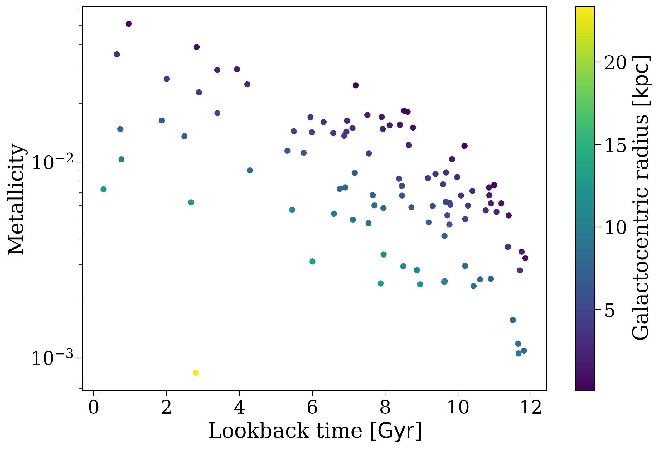
One could imagine using this to select out only certain systems that formed in particular locations or at particular times.
Stellar Evolution Information#
These are the main outputs from COSMIC, each table is a pandas DataFrame which is indexed by the unique binary number. For more details on exactly what each column in the tables mean you should refer to the relevant documentation from COSMIC.
bpp - Evolutionary table#
This table has, for each binary (or single star if you kept them), a row for every key evolutionary change in the history of the binary. These are listed on the COSMIC docs but you can also just use the cogsworth translator to get a full list of them:
[13]:
from cogsworth.utils import evol_type_translator
[evol_type_translator[i]["long"] for i in range(1, len(evol_type_translator))]
[13]:
['Initial state',
 'Stellar type changed',
 'Roche lobe overflow started',
 'Roche lobe overflow ended',
 'Binary entered contact phase',
 'Binary coalesced',
 'Common-envelope started',
 'Common-envelope ended',
 'No remnant',
 'Maximum evolution time reached',
 'Binary disrupted',
 'Begin symbiotic phase',
 'End symbiotic phase',
 'Blue straggler',
 'Supernova of primary',
 'Supernova of secondary']
Here’s an example set of rows for a certain binary (I’ll cherry-pick the most complicated one in this simulations)
[14]:
n_bpp_rows = np.array([len(p.bpp.loc[i]) for i in p.bin_nums])
complicated_binary = p.bin_nums[np.argmax(n_bpp_rows)]
p.bpp.loc[complicated_binary]
[14]:
| tphys | mass_1 | mass_2 | kstar_1 | kstar_2 | sep | porb | ecc | RRLO_1 | RRLO_2 | evol_type | aj_1 | aj_2 | tms_1 | tms_2 | massc_he_layer_1 | massc_he_layer_2 | massc_co_layer_1 | massc_co_layer_2 | rad_1 | rad_2 | mass0_1 | mass0_2 | lum_1 | lum_2 | teff_1 | teff_2 | radc_1 | radc_2 | menv_1 | menv_2 | renv_1 | renv_2 | omega_spin_1 | omega_spin_2 | B_1 | B_2 | bacc_1 | bacc_2 | tacc_1 | tacc_2 | epoch_1 | epoch_2 | bhspin_1 | bhspin_2 | bin_num | |
|---|---|---|---|---|---|---|---|---|---|---|---|---|---|---|---|---|---|---|---|---|---|---|---|---|---|---|---|---|---|---|---|---|---|---|---|---|---|---|---|---|---|---|---|---|---|---|
| 30 | 0.000000 | 3.346758 | 3.280125 | 1 | 1 | 14.503716 | 2.486775 | 0.23148 | 0.531995 | 0.530901 | 1 | 0.000000 | 0.000000 | 297.538628 | 3.141252e+02 | 0.000000 | 0.000000 | 0.000000 | 0.000000 | 2.257264 | 2.232016 | 3.346758 | 3.280125 | 118.558016 | 109.749412 | 12733.892916 | 12560.922079 | 0.000000 | 0.000000 | 1.000000e-10 | 1.000000e-10 | 1.000000e-10 | 1.000000e-10 | 5976.438387 | 6056.826731 | 0.0 | 0.0 | 0.0 | 0.0 | 0.0 | 0.0 | 0.000000 | 0.000000 | 0.0 | 0.0 | 30 |
| 30 | 276.138024 | 3.346650 | 3.280110 | 1 | 1 | 13.928341 | 2.340295 | 0.00000 | 1.001368 | 0.901218 | 3 | 276.139935 | 276.137965 | 297.564613 | 3.141291e+02 | 0.000000 | 0.000000 | 0.000000 | 0.000000 | 5.309222 | 4.734580 | 3.346650 | 3.280110 | 208.500118 | 184.539179 | 9561.603793 | 9820.893812 | 0.000000 | 0.000000 | 1.000000e-10 | 1.000000e-10 | 1.000000e-10 | 1.000000e-10 | 980.590253 | 980.590253 | 0.0 | 0.0 | 0.0 | 0.0 | 0.0 | 0.0 | -0.001911 | 0.000060 | 0.0 | 0.0 | 30 |
| 30 | 300.517503 | 2.811980 | 3.814779 | 1 | 1 | 14.641562 | 2.522334 | 0.00000 | 0.999489 | 0.800528 | 4 | 478.126863 | 176.357197 | 478.956468 | 2.100593e+02 | 0.000000 | 0.000000 | 0.000000 | 0.000000 | 5.163515 | 4.753789 | 2.811980 | 3.814779 | 130.895249 | 331.585237 | 8630.339051 | 11347.454183 | 0.000000 | 0.000000 | 1.000000e-10 | 1.000000e-10 | 1.000000e-10 | 1.000000e-10 | 905.935025 | 1026.772110 | 0.0 | 0.0 | 0.0 | 0.0 | 0.0 | 0.0 | -177.609360 | 124.160306 | 0.0 | 0.0 | 30 |
| 30 | 301.347108 | 2.811980 | 3.814779 | 2 | 1 | 14.693061 | 2.535654 | 0.00000 | 0.919890 | 0.803176 | 2 | 478.956468 | 177.186802 | 478.956468 | 2.100593e+02 | 0.375444 | 0.000000 | 0.000000 | 0.000000 | 4.769011 | 4.786291 | 2.811980 | 3.814779 | 145.464131 | 332.710999 | 9220.286982 | 11318.447639 | 0.075532 | 0.000000 | 1.000000e-10 | 1.000000e-10 | 1.000000e-10 | 1.000000e-10 | 1169.568958 | 963.671991 | 0.0 | 0.0 | 0.0 | 0.0 | 0.0 | 0.0 | -177.609360 | 124.160306 | 0.0 | 0.0 | 30 |
| 30 | 301.546529 | 2.811970 | 3.814782 | 2 | 1 | 14.713398 | 2.540922 | 0.00000 | 1.000107 | 0.803392 | 3 | 479.160622 | 177.385862 | 478.961200 | 2.100589e+02 | 0.376052 | 0.000000 | 0.000000 | 0.000000 | 5.192051 | 4.794205 | 2.811970 | 3.814782 | 138.311098 | 332.983634 | 8725.983389 | 11311.417426 | 0.075727 | 0.000000 | 1.000000e-10 | 1.000000e-10 | 1.000000e-10 | 1.000000e-10 | 903.164653 | 903.164653 | 0.0 | 0.0 | 0.0 | 0.0 | 0.0 | 0.0 | -177.614093 | 124.160667 | 0.0 | 0.0 | 30 |
| 30 | 304.343311 | 0.933813 | 5.692601 | 3 | 1 | 47.752406 | 14.856817 | 0.00000 | 1.863496 | 0.168796 | 2 | 499.802143 | 45.098005 | 496.775451 | 7.693055e+01 | 0.376655 | 0.000000 | 0.000000 | 0.000000 | 21.198332 | 4.333607 | 2.775261 | 5.692601 | 66.249688 | 1238.210355 | 3592.648449 | 16521.270341 | 0.075919 | 0.000000 | 2.785789e-01 | 1.000000e-10 | 1.372957e+01 | 1.000000e-10 | 316.606083 | 5235.414810 | 0.0 | 0.0 | 0.0 | 0.0 | 0.0 | 0.0 | -195.458832 | 259.245306 | 0.0 | 0.0 | 30 |
| 30 | 308.108632 | 0.412911 | 6.211860 | 3 | 1 | 192.816398 | 120.559840 | 0.00000 | 0.966466 | 0.038999 | 4 | 503.567464 | 37.115325 | 496.775451 | 6.267845e+01 | 0.406537 | 0.000000 | 0.000000 | 0.000000 | 34.166034 | 4.582352 | 2.775261 | 6.211860 | 372.510274 | 1714.399216 | 4357.695581 | 17428.233850 | 0.085140 | 0.000000 | 1.000000e-10 | 1.000000e-10 | 1.000000e-10 | 1.000000e-10 | 19.349164 | 5027.517162 | 0.0 | 0.0 | 0.0 | 0.0 | 0.0 | 0.0 | -195.458832 | 270.993307 | 0.0 | 0.0 | 30 |
| 30 | 308.339047 | 0.412011 | 6.212447 | 4 | 1 | 192.789886 | 120.537830 | 0.00000 | 0.182860 | 0.039124 | 2 | 503.797878 | 37.337610 | 496.775451 | 6.266475e+01 | 0.408365 | 0.000000 | 0.000000 | 0.000000 | 6.459117 | 4.597698 | 2.775261 | 6.212447 | 448.534153 | 1720.948081 | 10498.612773 | 17415.715219 | 0.085685 | 0.000000 | 1.000000e-10 | 1.000000e-10 | 1.000000e-10 | 1.000000e-10 | 54.689954 | 4992.929854 | 0.0 | 0.0 | 0.0 | 0.0 | 0.0 | 0.0 | -195.458832 | 271.001436 | 0.0 | 0.0 | 30 |
| 30 | 310.250458 | 0.411497 | 6.211483 | 7 | 1 | 192.825196 | 120.584403 | 0.00000 | 0.002471 | 0.040227 | 2 | 4.763431 | 39.262812 | 308.634442 | 6.268727e+01 | 0.408449 | 0.000000 | 0.003047 | 0.000000 | 0.087261 | 4.728770 | 0.411497 | 6.211483 | 7.247109 | 1771.005901 | 32203.355275 | 17296.193427 | 0.000000 | 0.000000 | 1.000000e-10 | 1.000000e-10 | 1.000000e-10 | 1.000000e-10 | 1767.466756 | 4713.372778 | 0.0 | 0.0 | 0.0 | 0.0 | 0.0 | 0.0 | 305.487027 | 270.987646 | 0.0 | 0.0 | 30 |
| 30 | 333.752555 | 0.411426 | 6.191377 | 7 | 2 | 193.413455 | 121.321563 | 0.00000 | 0.002551 | 0.063842 | 2 | 28.277469 | 63.159652 | 308.857168 | 6.315962e+01 | 0.393353 | 1.126197 | 0.018073 | 0.000000 | 0.090436 | 7.524906 | 0.411426 | 6.191377 | 7.534752 | 3404.440400 | 31942.346931 | 16144.719652 | 0.000000 | 0.223691 | 3.933529e-01 | 1.000000e-10 | 9.043573e-02 | 1.000000e-10 | 677.423658 | 2216.519219 | 0.0 | 0.0 | 0.0 | 0.0 | 0.0 | 0.0 | 305.475087 | 270.592903 | 0.0 | 0.0 | 30 |
| 30 | 333.971101 | 0.411426 | 6.190846 | 7 | 3 | 187.401531 | 115.713801 | 0.00000 | 0.002633 | 0.790908 | 2 | 28.496065 | 63.390790 | 308.857731 | 6.317218e+01 | 0.393213 | 1.148648 | 0.018213 | 0.000000 | 0.090465 | 90.323498 | 0.411426 | 6.190846 | 7.537788 | 1677.673855 | 31940.328513 | 3904.326423 | 0.000000 | 0.226973 | 3.932131e-01 | 2.521731e+00 | 9.046538e-02 | 5.857064e+01 | 709.627654 | 12.628228 | 0.0 | 0.0 | 0.0 | 0.0 | 0.0 | 0.0 | 305.475035 | 270.580310 | 0.0 | 0.0 | 30 |
| 30 | 333.976480 | 0.411426 | 6.190819 | 7 | 3 | 152.342676 | 84.812276 | 0.00000 | 0.003239 | 1.001043 | 3 | 28.501430 | 63.396169 | 308.857572 | 6.317218e+01 | 0.393210 | 1.148711 | 0.018216 | 0.000000 | 0.090466 | 92.934255 | 0.411426 | 6.190846 | 7.537868 | 1747.945172 | 31940.281469 | 3888.782472 | 0.000000 | 0.226982 | 3.932097e-01 | 2.626190e+00 | 9.046613e-02 | 6.161289e+01 | 27.058236 | 27.058236 | 0.0 | 0.0 | 0.0 | 0.0 | 0.0 | 0.0 | 305.475050 | 270.580310 | 0.0 | 0.0 | 30 |
| 30 | 333.976480 | 0.411426 | 6.190819 | 7 | 3 | 152.342676 | 84.812276 | 0.00000 | 0.003239 | 1.001043 | 7 | 28.501430 | 63.396169 | 308.857572 | 6.317218e+01 | 0.393210 | 1.148711 | 0.018216 | 0.000000 | 0.090466 | 92.934255 | 0.411426 | 6.190846 | 7.537868 | 1747.945172 | 31940.281469 | 3888.782472 | 0.000000 | 0.226982 | 3.932097e-01 | 2.626190e+00 | 9.046613e-02 | 6.161289e+01 | 27.058236 | 27.058236 | 0.0 | 0.0 | 0.0 | 0.0 | 0.0 | 0.0 | 305.475050 | 270.580310 | 0.0 | 0.0 | 30 |
| 30 | 333.976480 | 0.411426 | 1.148711 | 7 | 7 | 0.763592 | 0.061913 | 0.00000 | 0.003239 | 0.002445 | 8 | 28.501430 | 0.000000 | 308.857572 | 6.317218e+01 | 0.393210 | 1.148711 | 0.018216 | 0.000000 | 0.090466 | 0.226982 | 0.411426 | 1.148711 | 7.537868 | 398.221685 | 31940.281469 | 54363.220032 | 0.000000 | 0.000000 | 3.932097e-01 | 1.148711e+00 | 9.046613e-02 | 2.269820e-01 | 27.058236 | 27.058236 | 0.0 | 0.0 | 0.0 | 0.0 | 0.0 | 0.0 | 305.475050 | 270.580310 | 0.0 | 0.0 | 30 |
| 30 | 333.976480 | 0.411426 | 1.148711 | 7 | 7 | 0.763592 | 0.061913 | 0.00000 | 0.402318 | 0.632872 | 4 | 28.501430 | 0.000000 | 308.857572 | 1.519689e+01 | 0.393210 | 1.148711 | 0.018216 | 0.000000 | 0.090466 | 0.226982 | 0.411426 | 1.148711 | 7.537868 | 398.221685 | 31940.281469 | 54363.220032 | 0.000000 | 0.000000 | 3.932097e-01 | 1.148711e+00 | 9.046613e-02 | 2.269820e-01 | 27.058236 | 36.077648 | 0.0 | 0.0 | 0.0 | 0.0 | 0.0 | 0.0 | 305.475050 | 333.976480 | 0.0 | 0.0 | 30 |
| 30 | 349.587774 | 0.412713 | 1.116370 | 7 | 8 | 0.676248 | 0.052121 | 0.00000 | 0.463166 | 0.703921 | 2 | 43.617492 | 16.240287 | 304.837395 | 1.624025e+01 | 0.384376 | 0.643889 | 0.028337 | 0.472481 | 0.093001 | 0.222246 | 0.412713 | 1.116370 | 7.899412 | 798.771414 | 31873.120979 | 65381.946270 | 0.000000 | 0.073330 | 3.843760e-01 | 1.000000e-10 | 9.300096e-02 | 1.000000e-10 | 2055.492403 | 37141.408526 | 0.0 | 0.0 | 0.0 | 0.0 | 0.0 | 0.0 | 305.970282 | 333.347486 | 0.0 | 0.0 | 30 |
| 30 | 350.541840 | 0.412999 | 1.110000 | 7 | 8 | 0.666055 | 0.051049 | 0.00000 | 0.470586 | 1.000987 | 3 | 44.443703 | 17.194354 | 303.956056 | 1.624025e+01 | 0.384020 | 0.543494 | 0.028979 | 0.566505 | 0.093222 | 0.310894 | 0.412999 | 1.116370 | 7.943495 | 1979.348179 | 31879.615252 | 69357.563539 | 0.000000 | 0.066203 | 3.840202e-01 | 1.000000e-10 | 9.322210e-02 | 1.000000e-10 | 44954.251934 | 44954.251934 | 0.0 | 0.0 | 0.0 | 0.0 | 0.0 | 0.0 | 306.098137 | 333.347486 | 0.0 | 0.0 | 30 |
| 30 | 350.895256 | 0.451625 | 1.064303 | 7 | 8 | 0.603548 | 0.044137 | 0.00000 | 0.553387 | 1.843034 | 5 | 31.311456 | 17.542305 | 220.357807 | 1.624025e+01 | 0.419699 | 0.428001 | 0.031926 | 0.640766 | 0.103596 | 0.512945 | 0.451625 | 1.116370 | 11.788351 | 3664.378540 | 33378.090300 | 62984.617317 | 0.000000 | 0.061200 | 4.157010e-01 | 1.000000e-10 | 1.035959e-01 | 1.000000e-10 | 130263.836557 | 33558.186105 | 0.0 | 0.0 | 0.0 | 0.0 | 0.0 | 0.0 | 319.578335 | 333.347486 | 0.0 | 0.0 | 30 |
| 30 | 350.895256 | 0.451625 | 1.064303 | 7 | 8 | 0.603548 | 0.044137 | 0.00000 | 0.553387 | 1.843034 | 7 | 31.311456 | 17.542305 | 220.357807 | 1.624025e+01 | 0.419699 | 0.428001 | 0.031926 | 0.640766 | 0.103596 | 0.512945 | 0.451625 | 1.116370 | 11.788351 | 3664.378540 | 33378.090300 | 62984.617317 | 0.000000 | 0.061200 | 4.157010e-01 | 1.000000e-10 | 1.035959e-01 | 1.000000e-10 | 130263.836557 | 33558.186105 | 0.0 | 0.0 | 0.0 | 0.0 | 0.0 | 0.0 | 319.578335 | 333.347486 | 0.0 | 0.0 | 30 |
| 30 | 350.895256 | 0.000000 | 1.492645 | 15 | 8 | 0.000000 | 0.000000 | 0.00000 | 0.553387 | 0.990000 | 8 | 31.311456 | 7.846723 | 220.357807 | 1.624025e+01 | 0.419705 | 0.819961 | 0.031921 | 0.672683 | 0.103596 | 0.512945 | 0.451625 | 1.545753 | 11.788351 | 3664.378540 | 33378.090300 | 62984.617317 | 0.000000 | 0.061200 | 4.157010e-01 | 1.000000e-10 | 1.035959e-01 | 1.000000e-10 | 130263.836557 | 33558.186105 | 0.0 | 0.0 | 0.0 | 0.0 | 0.0 | 0.0 | 319.578335 | 333.347486 | 0.0 | 0.0 | 30 |
| 30 | 351.594240 | 0.000000 | 1.447840 | 15 | 9 | 0.000000 | 0.000000 | -1.00000 | -1.000000 | 0.000100 | 2 | 31.311456 | 8.545708 | 220.357807 | 7.846723e+00 | 0.000000 | 0.479485 | 0.000000 | 0.968355 | 0.103596 | 104.406973 | 0.451625 | 1.545753 | 11.788351 | 14262.183564 | 33378.090300 | 6200.851983 | 0.000000 | 0.042068 | 4.157010e-01 | 4.794851e-01 | 1.035959e-01 | 1.043649e+02 | 130263.836557 | 0.775681 | 0.0 | 0.0 | 0.0 | 0.0 | 0.0 | 0.0 | 319.583800 | 343.048533 | 0.0 | 0.0 | 30 |
| 30 | 351.745898 | 0.000000 | 0.630980 | 15 | 11 | 0.000000 | 0.000000 | -1.00000 | -1.000000 | 0.000100 | 2 | 31.311456 | 0.000000 | 220.357807 | 7.846723e+00 | 0.000000 | 0.000000 | 0.000000 | 0.000000 | 0.103596 | 0.012367 | 0.451625 | 0.604922 | 11.788351 | 23.947382 | 33378.090300 | 115331.888084 | 0.000000 | 0.012367 | 4.157010e-01 | 1.000000e-10 | 1.035959e-01 | 1.000000e-10 | 130263.836557 | 0.000005 | 0.0 | 0.0 | 0.0 | 0.0 | 0.0 | 0.0 | 319.583800 | 351.745898 | 0.0 | 0.0 | 30 |
| 30 | 2891.512981 | 0.000000 | 0.630980 | 15 | 11 | 0.000000 | 0.000000 | -1.00000 | -1.000000 | 0.000100 | 10 | 31.311456 | 2539.767083 | 220.357807 | 1.000000e+10 | 0.000000 | 0.000000 | 0.000000 | 0.000000 | 0.103596 | 0.012367 | 0.451625 | 0.604922 | 11.788351 | 0.000152 | 33378.090300 | 5788.021776 | 0.000000 | 0.012367 | 4.157010e-01 | 1.000000e-10 | 1.035959e-01 | 1.000000e-10 | 130263.836557 | 0.000005 | 0.0 | 0.0 | 0.0 | 0.0 | 0.0 | 0.0 | 319.583800 | 351.745898 | 0.0 | 0.0 | 30 |
Now that table was probably a little hard to parse if you’re not familiar with COSMIC or BSE output because they have numbers for each stellar type and evolutionary phase. Don’t worry, you don’t need to remember what these numbers mean because cogsworth can translate the table for you
[15]:
p.translate_tables(label_type="long", replace_columns=False)
[16]:
p.bpp.loc[complicated_binary][["tphys", "evol_type_str", "mass_1", "mass_2", "kstar_1_str", "kstar_2_str", "sep", "porb", "ecc"]]
[16]:
| tphys | evol_type_str | mass_1 | mass_2 | kstar_1_str | kstar_2_str | sep | porb | ecc | |
|---|---|---|---|---|---|---|---|---|---|
| 30 | 0.000000 | Initial state | 3.346758 | 3.280125 | Main Sequence | Main Sequence | 14.503716 | 2.486775 | 0.23148 |
| 30 | 276.138024 | Roche lobe overflow started | 3.346650 | 3.280110 | Main Sequence | Main Sequence | 13.928341 | 2.340295 | 0.00000 |
| 30 | 300.517503 | Roche lobe overflow ended | 2.811980 | 3.814779 | Main Sequence | Main Sequence | 14.641562 | 2.522334 | 0.00000 |
| 30 | 301.347108 | Stellar type changed | 2.811980 | 3.814779 | Hertzsprung Gap | Main Sequence | 14.693061 | 2.535654 | 0.00000 |
| 30 | 301.546529 | Roche lobe overflow started | 2.811970 | 3.814782 | Hertzsprung Gap | Main Sequence | 14.713398 | 2.540922 | 0.00000 |
| 30 | 304.343311 | Stellar type changed | 0.933813 | 5.692601 | First Giant Branch | Main Sequence | 47.752406 | 14.856817 | 0.00000 |
| 30 | 308.108632 | Roche lobe overflow ended | 0.412911 | 6.211860 | First Giant Branch | Main Sequence | 192.816398 | 120.559840 | 0.00000 |
| 30 | 308.339047 | Stellar type changed | 0.412011 | 6.212447 | Core Helium Burning | Main Sequence | 192.789886 | 120.537830 | 0.00000 |
| 30 | 310.250458 | Stellar type changed | 0.411497 | 6.211483 | Helium Main Sequence | Main Sequence | 192.825196 | 120.584403 | 0.00000 |
| 30 | 333.752555 | Stellar type changed | 0.411426 | 6.191377 | Helium Main Sequence | Hertzsprung Gap | 193.413455 | 121.321563 | 0.00000 |
| 30 | 333.971101 | Stellar type changed | 0.411426 | 6.190846 | Helium Main Sequence | First Giant Branch | 187.401531 | 115.713801 | 0.00000 |
| 30 | 333.976480 | Roche lobe overflow started | 0.411426 | 6.190819 | Helium Main Sequence | First Giant Branch | 152.342676 | 84.812276 | 0.00000 |
| 30 | 333.976480 | Common-envelope started | 0.411426 | 6.190819 | Helium Main Sequence | First Giant Branch | 152.342676 | 84.812276 | 0.00000 |
| 30 | 333.976480 | Common-envelope ended | 0.411426 | 1.148711 | Helium Main Sequence | Helium Main Sequence | 0.763592 | 0.061913 | 0.00000 |
| 30 | 333.976480 | Roche lobe overflow ended | 0.411426 | 1.148711 | Helium Main Sequence | Helium Main Sequence | 0.763592 | 0.061913 | 0.00000 |
| 30 | 349.587774 | Stellar type changed | 0.412713 | 1.116370 | Helium Main Sequence | Helium Hertsprung Gap | 0.676248 | 0.052121 | 0.00000 |
| 30 | 350.541840 | Roche lobe overflow started | 0.412999 | 1.110000 | Helium Main Sequence | Helium Hertsprung Gap | 0.666055 | 0.051049 | 0.00000 |
| 30 | 350.895256 | Binary entered contact phase | 0.451625 | 1.064303 | Helium Main Sequence | Helium Hertsprung Gap | 0.603548 | 0.044137 | 0.00000 |
| 30 | 350.895256 | Common-envelope started | 0.451625 | 1.064303 | Helium Main Sequence | Helium Hertsprung Gap | 0.603548 | 0.044137 | 0.00000 |
| 30 | 350.895256 | Common-envelope ended | 0.000000 | 1.492645 | Massless Remnant | Helium Hertsprung Gap | 0.000000 | 0.000000 | 0.00000 |
| 30 | 351.594240 | Stellar type changed | 0.000000 | 1.447840 | Massless Remnant | Helium Giant Branch | 0.000000 | 0.000000 | -1.00000 |
| 30 | 351.745898 | Stellar type changed | 0.000000 | 0.630980 | Massless Remnant | Carbon/Oxygen White Dwarf | 0.000000 | 0.000000 | -1.00000 |
| 30 | 2891.512981 | Maximum evolution time reached | 0.000000 | 0.630980 | Massless Remnant | Carbon/Oxygen White Dwarf | 0.000000 | 0.000000 | -1.00000 |
A tad less brain-melting no?
Tip
You can change the style of these translations (between “short” and “long”) and also elect to overwrite the original columns to save memory (but you’ll only want to do that once you’re done masking probably)
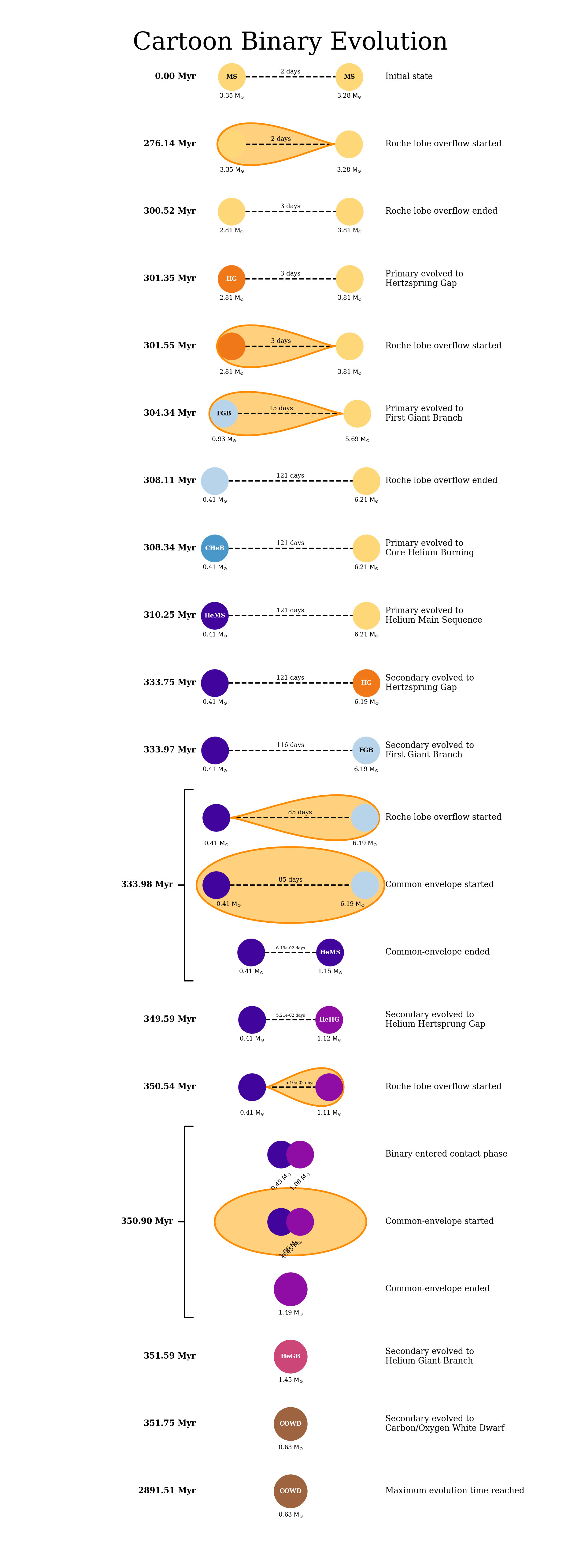
If you’re more of a visual person you can also convert this whole table into an evolution cartoon with some of the cogsworth utilities. Let’s do this for the complicated binary we found
[17]:
p.plot_cartoon_binary(complicated_binary);
bcm - User-specified timestep table#
The columns here are identical to the bpp table and by default, this table will only include timesteps for the start and end of the evolution of each binary (and thus we don’t save it in cogsworth in these cases). However, you can use bcm_timestep_conditions to define particular conditions that can result in finer resolution timestep conditions being printed. For example you could print extra timesteps for any binary that is transferring mass onto a compact object to look at X-ray binaries in more detail.
For more details on this check out the cogsworth tutorial on re-running binaries and the COSMIC docs about the setting the time resolution dynamically.
kick_info - Supernova kick information#
This table contains two rows per binary, displaying the info for the two potential supernova kicks that may occur for each star. The columns tell you about the magnitude and direction of the kicks as well as the impact on the systemic velocity.
Here’s the table for the systems that actually received kicks
[18]:
p.kick_info.loc[p.kick_info[p.kick_info["natal_kick"] > 0.0]["bin_num"].unique()]
[18]:
| star | disrupted | natal_kick | phi | theta | mean_anomaly | delta_vsysx_1 | delta_vsysy_1 | delta_vsysz_1 | vsys_1_total | delta_vsysx_2 | delta_vsysy_2 | delta_vsysz_2 | vsys_2_total | theta_euler | phi_euler | psi_euler | randomseed | bin_num | |
|---|---|---|---|---|---|---|---|---|---|---|---|---|---|---|---|---|---|---|---|
| 2 | 1.0 | 1.0 | 97.322127 | -24.636763 | 124.831960 | 0.000000 | -50.527420 | 72.612968 | -40.570100 | 97.322127 | 0.000000 | 0.000000 | 0.000000 | 0.000000 | 0.000000 | 0.000000 | 0.000000 | -5.145293e+08 | 2.0 |
| 2 | 0.0 | 0.0 | 0.000000 | 0.000000 | 0.000000 | 0.000000 | 0.000000 | 0.000000 | 0.000000 | 0.000000 | 0.000000 | 0.000000 | 0.000000 | 0.000000 | 0.000000 | 0.000000 | 0.000000 | 0.000000e+00 | 2.0 |
| 3 | 1.0 | 1.0 | 63.416925 | 6.800539 | 106.803696 | 333.993301 | -21.713766 | 69.550218 | 5.214060 | 73.047292 | -0.487510 | -5.310271 | 0.751388 | 5.385279 | 6.643533 | 226.651983 | 337.185280 | -9.541407e+08 | 3.0 |
| 3 | 2.0 | 1.0 | 179.721303 | 40.915287 | 292.643380 | 0.000000 | 0.000000 | 0.000000 | 0.000000 | 73.047292 | 52.286667 | -125.343078 | 117.707111 | 183.809321 | 0.000000 | 0.000000 | 0.000000 | 7.436287e+08 | 3.0 |
| 6 | 1.0 | 1.0 | 389.914739 | 52.900686 | 198.333735 | 0.000000 | -223.257518 | -73.981224 | 310.992545 | 389.914739 | 0.000000 | 0.000000 | 0.000000 | 0.000000 | 0.000000 | 0.000000 | 0.000000 | -1.725820e+09 | 6.0 |
| ... | ... | ... | ... | ... | ... | ... | ... | ... | ... | ... | ... | ... | ... | ... | ... | ... | ... | ... | ... |
| 97 | 0.0 | 0.0 | 0.000000 | 0.000000 | 0.000000 | 0.000000 | 0.000000 | 0.000000 | 0.000000 | 0.000000 | 0.000000 | 0.000000 | 0.000000 | 0.000000 | 0.000000 | 0.000000 | 0.000000 | 0.000000e+00 | 97.0 |
| 98 | 1.0 | 1.0 | 126.484524 | 12.444072 | 28.004209 | 308.889477 | 124.991380 | 85.662558 | 25.550593 | 153.667666 | -4.957441 | -5.871536 | 0.215610 | 7.687499 | 9.075057 | 97.549260 | 136.397753 | -6.192077e+08 | 98.0 |
| 98 | 2.0 | 1.0 | 93.645108 | -5.015615 | 334.551909 | 0.000000 | 0.000000 | 0.000000 | 0.000000 | 153.667666 | 84.235402 | -40.084588 | -8.187133 | 91.981006 | 0.000000 | 0.000000 | 0.000000 | 2.051889e+09 | 98.0 |
| 99 | 1.0 | 1.0 | 1172.966666 | 32.163143 | 21.069551 | 0.000000 | 926.573748 | 356.969440 | 624.407485 | 1172.966666 | 0.000000 | 0.000000 | 0.000000 | 0.000000 | 0.000000 | 0.000000 | 0.000000 | -8.935563e+08 | 99.0 |
| 99 | 0.0 | 0.0 | 0.000000 | 0.000000 | 0.000000 | 0.000000 | 0.000000 | 0.000000 | 0.000000 | 0.000000 | 0.000000 | 0.000000 | 0.000000 | 0.000000 | 0.000000 | 0.000000 | 0.000000 | 0.000000e+00 | 99.0 |
130 rows × 19 columns
Galactic Evolution Information#
So now you know how everything started and how each binary system evolved, the last outputs now tell you the path each system took through the galaxy and where they ended.
orbits - Galactic orbits#
The full tracks are stored in orbits, there is an orbit entry for every bound binary and each disrupted primary/secondary. Because this has a slightly strange shape you can access these orbits more easily as primary_orbits and secondary_orbits, which return the orbits of the binaries for bound systems and individual stars in disrupted systems.
First let’s look at the orbit of a bound binary
[19]:
fig, ax = plt.subplots()
bound_orbits = p.primary_orbits[~p.disrupted]
np.random.choice(bound_orbits).plot(['x', 'y'], axes=[ax])
plt.show()
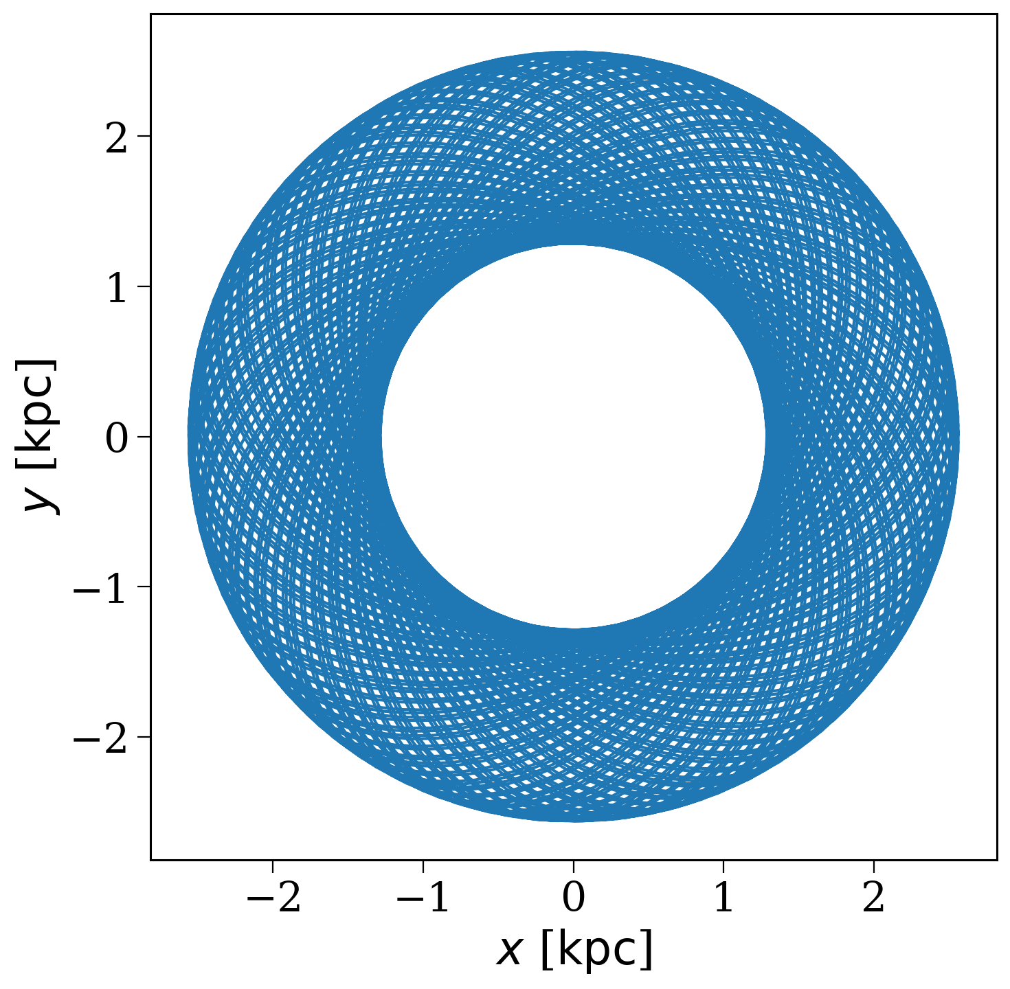
Tip
Try changing that last cell to use secondary_orbits - you’ll note the plot looks identical because this is a bound binary and the secondary is going to follow the same track as the primary
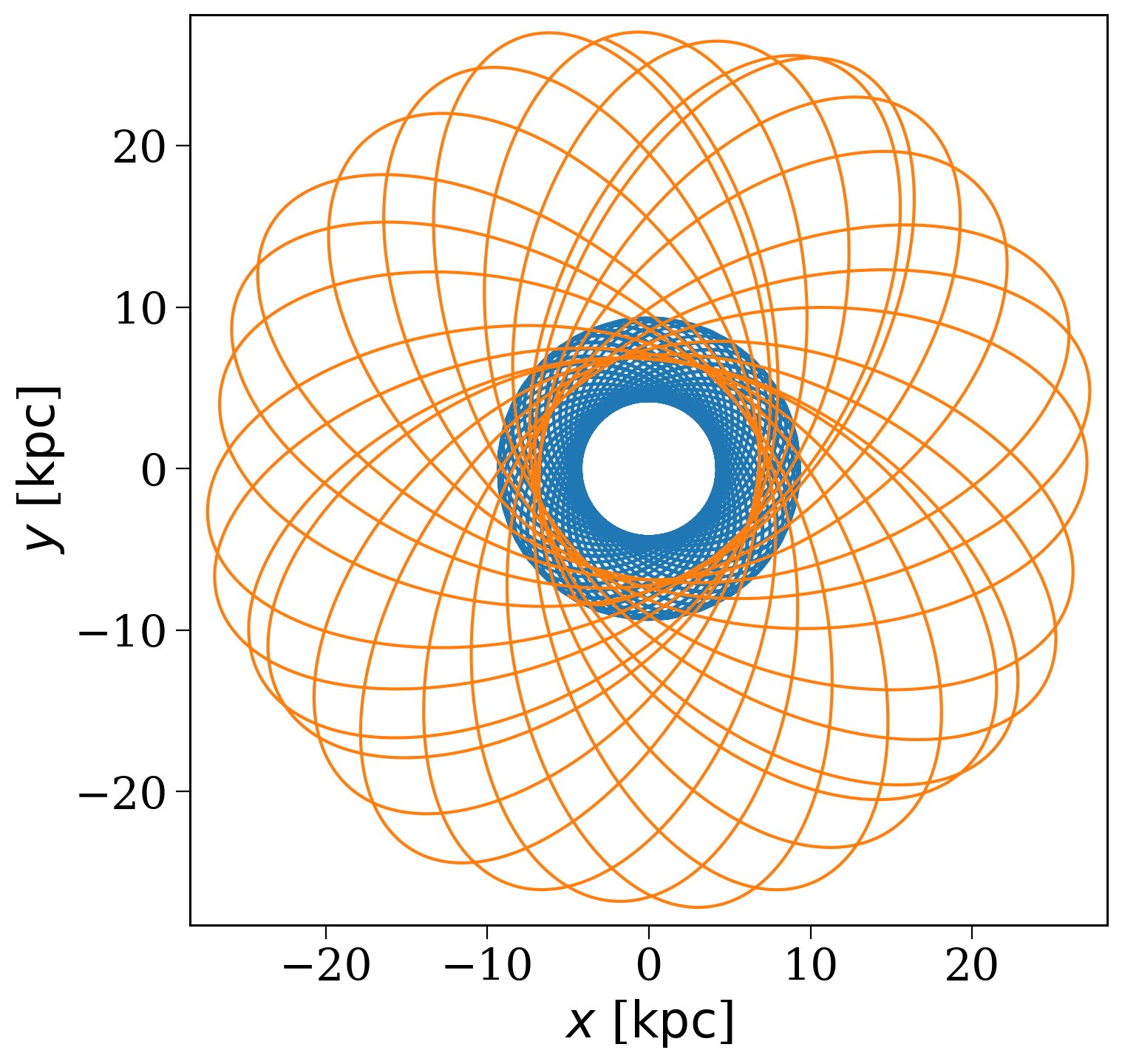
And now let’s pick a random disrupted system
[25]:
fig, ax = plt.subplots()
random_disrupted_ind = np.random.randint(p.disrupted.sum())
p.primary_orbits[p.disrupted][random_disrupted_ind].plot(['x', 'y'], axes=[ax])
p.secondary_orbits[p.disrupted][random_disrupted_ind].plot(['x', 'y'], axes=[ax])
plt.show()
final_pos,vel - Final states#
A lot of the time you might not need the full orbit and actually only care where the system is at the end of the simulation (and how it is moving). In this case you don’t need to access each orbit but can instead just use final_pos/vel. These arrays both have the same length as orbits but now with the 3 dimensions each.
[21]:
p.final_pos
[21]:
[22]:
p.final_vel
[22]:
Wrap-up#
And that’s all for this one! Hopefully you now have a better understanding of the outputs of a cogsworth simulation and how to interpret them. Keep reading in the next tutorial to learn about how to save and load simulations, and check out the other tutorials to see all of the features of cogsworth!
Note
This tutorial was generated from a Jupyter notebook that can be found here.