Plotting potentials and orbits

cogsworth combines population synthesis with galactic dynamics done with gala. Though the gala documentation of course will give a comprehensive overview, in this tutorial I’ll highlight some very useful features and ways to visualise your outputs.

Learning Goals

By the end of this tutorial you should know how to:

• Calculate simple values for Potentials (such as MilkyWayPotential), like escape velocities

• Plot and animate an Orbit

• Learn to use the cogsworth plot_orbit() function

• Read the gala docs for proper details ;)

import cogsworth
import matplotlib.pyplot as plt
import numpy as np
import pandas as pd
import astropy.units as u

# this all just makes plots look nice
%config InlineBackend.figure_format = 'retina'

plt.rc('font', family='serif')
plt.rcParams['text.usetex'] = False
fs = 24

# update various fontsizes to match
params = {'figure.figsize': (12, 8),
          'legend.fontsize': fs,
          'axes.labelsize': fs,
          'xtick.labelsize': 0.9 * fs,
          'ytick.labelsize': 0.9 * fs,
          'axes.linewidth': 1.1,
          'xtick.major.size': 7,
          'xtick.minor.size': 4,
          'ytick.major.size': 7,
          'ytick.minor.size': 4}
plt.rcParams.update(params)
pd.options.display.max_columns = 999

Potentials

Tip

This is just a preview of some of the capabilities, for more detailed documentation of Potentials check out the Gala Potential docs!

Let’s first focus on potentials. Each cogsworth population requires a galactic_potential attribute to perform galactic orbit integrations. These potentials are specified as gala PotentialBase classes, which come with some very useful functionality.

Let’s try it out with the default Milky Way potential used in cogsworth.

p = cogsworth.pop.Population(100, final_kstar1=[14], timestep_size=0.1 * u.Myr,
                             use_default_BSE_settings=True)
p.galactic_potential

<CompositePotential disk,bulge,nucleus,halo>

As you can see, this is a composite potential and several components and each can be accessed and operated on individually.

p.galactic_potential["disk"]

<MN3ExponentialDiskPotential: m=4.77e+10 solMass, h_R=2.60 kpc, h_z=0.30 kpc (kpc,Myr,solMass,rad)>

For any potential you can query all sorts of information from Gala - for example you can get the circular velocity at any given location as follows.

p.galactic_potential.circular_velocity(q=[8.5, 0, 0] * u.kpc)

$[228.89326] \; \mathrm{\frac{km}{s}}$

One useful aspect for visualisation can be showing the equipotential contours for each potential. For this you just need to specify the grid upon which to evaluate the potential in the certain projection you’re interested in.

Let’s do this for the $x$-$y$ (face on) and $x$-$z$ (edge on) projections for the inner 5 kpc.

fig, axes = plt.subplots(1, 2, figsize=(20, 10))

# define a basic grid to use
grid = np.linspace(-5, 5, 100) * u.kpc

# plot using the grid for x, y, but fixing z=0 kpc (repeat for x-z with y=0)
p.galactic_potential.plot_contours(grid=(grid, grid, 0), ax=axes[0]);
p.galactic_potential.plot_contours(grid=(grid, 0, grid), ax=axes[1]);

axes[0].set(xlabel=r'$x \, [\rm kpc]$', ylabel=r'$y \, [\rm kpc]$')
axes[1].set(xlabel=r'$x \, [\rm kpc]$', ylabel=r'$z \, [\rm kpc]$')

plt.show()

Orbits

Tip

This is just a preview of some of the capabilities, for more detailed documentation of Orbits check out the Gala Orbit docs!

After performing galactic evolution, for each binary cogsworth will store an orbit (or two if it disrupted) in p.orbits. These orbits essentially just contain arrays of positions and velocities for certain timesteps. However each comes with a lot of useful functionality.

Let’s fully evolve our population that we started earlier and investigate some orbits.

np.random.seed(27)
p.create_population(with_timing=False)
p.orbits[0]

cogsworth warning: 2 orbit(s) failed numerical integration, removing them. This can occur due to NaNs in stellar evolution or extreme orbits (e.g. passing directly through the galactic centre) that Gala cannot handle. Information for these systems was saved to `./failed_integration_binaries_2.h5`. This includes their initial_binaries, bpp, kick_info, and initial galaxy objects.

<Orbit cartesian, dim=3, shape=(77554,)>

As noted above, each orbit stores positions, velocities and times

p.orbits[0].pos, p.orbits[0].vel, p.orbits[0].t

(<CartesianRepresentation (x, y, z) in kpc
     [(   3.35032142, -11.84849161,  -0.25276921),
      (   3.37279179, -11.84225441,  -0.25271107),
      (   3.39525075, -11.83597714,  -0.25264944), ...,
      (1881.2970941 , 236.01257651, 216.97822302),
      (1881.31807053, 236.01547516, 216.98066842),
      (1881.33041451, 236.01718093, 216.98210746)]>,
 <CartesianDifferential (d_x, d_y, d_z) in kpc / Myr
     [(0.22476052, 0.06217164, 0.00056397),
      (0.22464678, 0.06257242, 0.00059887),
      (0.22453229, 0.06297299, 0.00063376), ...,
      (0.2097645 , 0.02898655, 0.02445397),
      (0.20976423, 0.02898652, 0.02445394),
      (0.20976408, 0.0289865 , 0.02445393)]>,
 <Quantity [ 4244.74115307,  4244.84115307,  4244.94115307, ...,
            11999.84115307, 11999.94115307, 12000.        ] Myr>)

You can also access specific coordinates as necessary

p.orbits[0].z

$[-0.25276921,~-0.25271107,~-0.25264944,~\dots,~216.97822,~216.98067,~216.98211] \; \mathrm{kpc}$

You can also transform your orbits between representations, for example let’s look at this orbit in cylindrical coordinates

p.orbits[0].cylindrical.rho

$[12.313058,~12.313193,~12.313329,~\dots,~1896.0434,~1896.0646,~1896.0771] \; \mathrm{kpc}$

And there’s lots of plotting options too, you can either plot the orbit in all cartesian projections (default) or specify coordinates you’re interested in.

plot_orbit = p.primary_orbits[~p.disrupted & ~p.escaped[:len(p)]][0]
plot_orbit.plot();

fig, ax = plt.subplots(figsize=(12, 7))
plot_orbit.cylindrical.plot(['rho', 'z'], axes=[ax]);

Disruption example

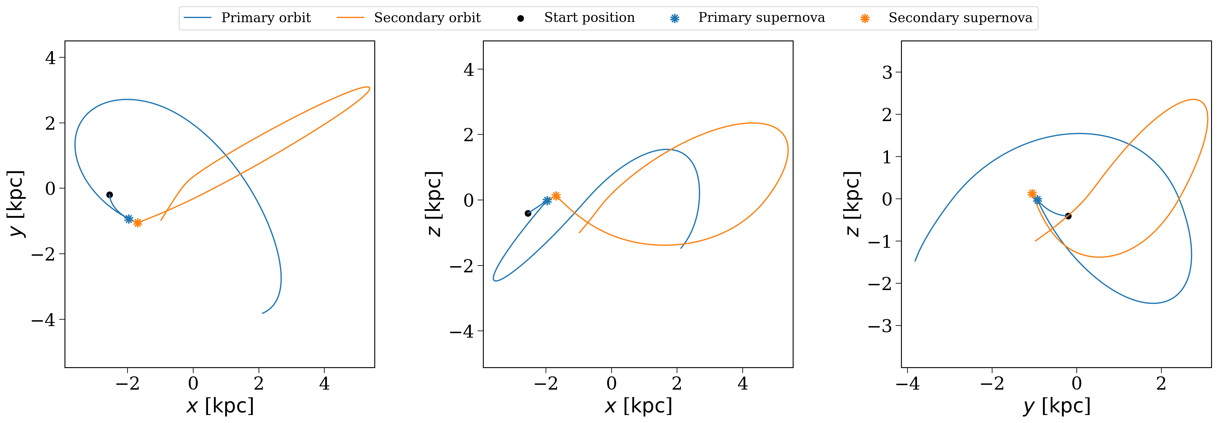
Let’s now do a more detailed example where we investigate the orbit of an interesting system that was disrupted by a supernova. We can plot both the primary and secondary orbit and see where things diverge.

So first let’s pick a subset of our population that’s interesting: something that has been disrupted, but that hasn’t escaped the galactic potential (straight lines aren’t pretty).

orbit_options_mask = p.disrupted & ~p.escaped[:len(p)]
orbit_options_bin_nums = p.bin_nums[orbit_options_mask]

Now let’s grab something that takes a significant excursion from the galactic plane…but not too far.

primary_orbit_options = p.primary_orbits[orbit_options_mask]
secondary_orbit_options = p.secondary_orbits[orbit_options_mask]
target_orbit = None
for i in range(len(primary_orbit_options)):
    if ((primary_orbit_options[i].z.max() > 1 * u.kpc)
        & (primary_orbit_options[i].z.max() < 10 * u.kpc)
        & (secondary_orbit_options[i].z.max() > 1 * u.kpc)
        & (secondary_orbit_options[i].z.max() < 10 * u.kpc)):
        target_ind = i
        break

Now let’s use cogsworth’s functionality for plotting both the primary and secondary orbits together.

p.plot_orbit(orbit_options_bin_nums[target_ind], show_sn=False);

Hmmm, okay well the primary and secondary orbit are definitely different, but this is a bit of a mess. Let’s try trimming to orbit to only slightly after the disruption occurs.

p.plot_orbit(orbit_options_bin_nums[target_ind], show_sn=True, t_max=100 * u.Myr);

Wrap-up

That’s all for this one! Remember that the gala documentation contains a lot more detail about this, these are just the most basic ways you might interact with potentials and orbits whilst using cogsworth!

Note

This tutorial was generated from a Jupyter notebook that can be found here.