Adding a time-evolving galactic potential

cogsworth allows you to change your galactic potential as a function of time, which can be important for long-lived objects. In this tutorial we’ll show how to do this and how it could affect the results for the distributions of NSs and BHs in the Milky Way.

Learning Goals

By the end of this tutorial you should know how to:

• Define a time-evolving galactic potential in cogsworth

• Understand how this can affect the results for the distributions of NSs and BHs in the Milky Way

import cogsworth
import matplotlib.pyplot as plt
import numpy as np
import pandas as pd
import astropy.units as u

import gala.potential as gp
import gala.dynamics as gd
from gala.units import galactic

# this all just makes plots look nice
%config InlineBackend.figure_format = 'retina'

plt.rc('font', family='serif')
plt.rcParams['text.usetex'] = False
fs = 24

# update various fontsizes to match
params = {'figure.figsize': (12, 8),
          'legend.fontsize': fs,
          'axes.labelsize': fs,
          'xtick.labelsize': 0.9 * fs,
          'ytick.labelsize': 0.9 * fs,
          'axes.linewidth': 1.1,
          'xtick.major.size': 7,
          'xtick.minor.size': 4,
          'ytick.major.size': 7,
          'ytick.minor.size': 4}
plt.rcParams.update(params)
pd.options.display.max_columns = 999

Defining an evolving potential

gala enables the time-evolution of potentials by performing interpolation between a set of potentials defined at different times. You can follow the detailed tutorial in gala on this (see here for more details), but let’s just cover the basic idea.

Let’s compare two NFW profiles, each which have the same final mass, but one of which starts with one tenth the mass and grows linerally.

static_nfw = gp.NFWPotential(m=1e12 * u.Msun, r_s=10 * u.kpc, units=galactic)
static_nfw

<NFWPotential: m=1.00e+12 solMass, r_s=10.00 kpc, a=1.00 , b=1.00 , c=1.00  (kpc,Myr,solMass,rad)>

time_knots = np.linspace(0, 12, 20) * u.Gyr
masses = np.linspace(1e11, 1e12, 20) * u.Msun
evolving_nfw = gp.TimeInterpolatedPotential(
    gp.NFWPotential, time_knots, m=masses, r_s=10 * u.kpc, units=galactic
)
evolving_nfw

<TimeInterpolatedPotential: NFWPotential interpolation_method='cspline')>

We can compare the orbits of a test particle in these two potentials. We’ll start with the same initial conditions for the test particle in both cases, and then integrate the orbits forward in time until present day.

w0 = gd.PhaseSpacePosition(
    pos=[8, 0, 0] * u.kpc,
    vel=[50, 50, -5] * u.km / u.s
)
w0

<PhaseSpacePosition cartesian, dim=3, shape=()>

orbits = [
    pot.integrate_orbit(w0, t1=0 * u.Gyr, t2=12 * u.Gyr, dt=1 * u.Myr, Integrator="DOPRI853")
    for pot in (static_nfw, evolving_nfw)
]

fig, axes = plt.subplots(1, 2, figsize=(12, 6))

for orbit, ax in zip(orbits, axes):
    scatter = ax.scatter(orbit.x, orbit.y, c=orbit.t.value, s=1)
    ax.annotate("Evolving NFW" if ax == axes[1] else "Static NFW", xy=(0.5, 0.0), xycoords='axes fraction',
                fontsize=12, ha='center', va='bottom')
    ax.set_aspect('equal')
    ax.set(
        xlim=(-10, 10),
        ylim=(-10, 10),
        xlabel='x (kpc)',
        ylabel='y (kpc)',
    )

fig.colorbar(scatter, ax=axes, label='Time (Myr)', orientation='horizontal', location="top")

plt.show()

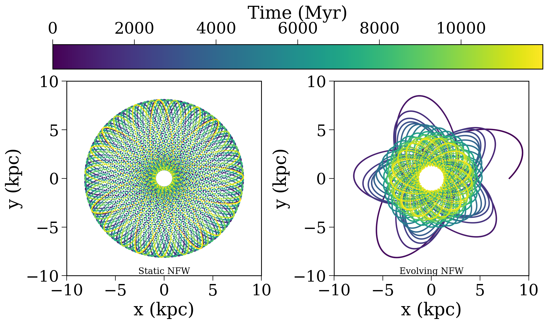
Clearly the orbits trace very different paths, which is not surprising given the very different potentials.

Evolving potentials in cogsworth

Now let’s see how we can use an evolving potential in cogsworth. The process is almost identical to how you would use a static potential, you just pass the defined evolving potential!

p = cogsworth.pop.Population(100, galactic_potential=evolving_nfw, use_default_BSE_settings=True)
p.create_population()

Run for 100 binaries
Sampled 131 binaries
[5e-03s] Sample initial binaries
[0.1s] Evolve binaries (run COSMIC)

Integrating orbits: 100%|██████████| 131/131 [00:00<00:00, 1524.37it/s]

[0.4s] Integrate galactic orbits (run gala)
Overall: 0.5s

Example: Escaping BHs and NSs

As an example, let’s look at how the distribution of NSs and BHs in the Milky Way changes when we use an evolving potential. We’ll start by defining a Milky Way potential that evolves over time, and then we’ll create a population of binaries using this evolving potential. Finally, we’ll compare the final positions of the NSs and BHs in this population to those in a population created using a static potential.

First, let’s define the evolving potential. Let’s assume everything starts with one tenth the mass of the Milky Way, and then grows linearly to the present day mass. This is a very simple model, but it will allow us to see how the results change when we use an evolving potential.

time_knots = np.linspace(0, 12, 5) * u.Gyr
mass_fractions = np.linspace(0.1, 1.0, 5)

evolving_mw = gp.CCompositePotential(
    disk=gp.TimeInterpolatedPotential(
        gp.MN3ExponentialDiskPotential,
        time_knots,
        m=6.8e10 * u.Msun * mass_fractions,
        h_R=2.6 * u.kpc,
        h_z=0.3 * u.kpc,
        units="galactic"
    ),
    bulge=gp.TimeInterpolatedPotential(
        gp.HernquistPotential,
        time_knots,
        m=5e9 * u.Msun * mass_fractions,
        c=1.0 * u.kpc,
        units="galactic"
    ),
    nucleus=gp.TimeInterpolatedPotential(
        gp.HernquistPotential,
        time_knots,
        m=1.81e9 * u.Msun * mass_fractions,
        c=0.07 * u.kpc,
        units="galactic"
    ),
    halo= gp.TimeInterpolatedPotential(
        gp.NFWPotential,
        time_knots,
        m=5.4e11 * u.Msun * mass_fractions,
        r_s=15.63 * u.kpc,
        units="galactic"
    )
)

Now we can use this to evolve a population of massive binaries. Let’s first evolve a population using the default Milky Way potential and then mask out the NSs and BHs. Then we can repeat with the evolving potential.

pop_static = cogsworth.pop.Population(
    2500, final_kstar1=[13, 14],
    galactic_potential=gp.MilkyWayPotential(version='v2'),
    use_default_BSE_settings=True
)
pop_static.create_population()

Run for 2500 binaries
Sampled 2549 binaries
[3e-02s] Sample initial binaries
[3.0s] Evolve binaries (run COSMIC)

Integrating orbits: 100%|██████████| 2741/2741 [00:03<00:00, 727.59it/s]
cogsworth warning: 3 orbit(s) failed numerical integration, removing them. This can occur due to NaNs in stellar evolution or extreme orbits (e.g. passing directly through the galactic centre) that Gala cannot handle. Information for these systems was saved to `./failed_integration_binaries_1.h5`. This includes their initial_binaries, bpp, kick_info, and initial galaxy objects.

[4.8s] Integrate galactic orbits (run gala)
Overall: 7.8s

pop_evolving = pop_static.copy()
pop_evolving.galactic_potential = evolving_mw
pop_evolving.perform_galactic_evolution()

Integrating orbits: 100%|██████████| 2738/2738 [00:26<00:00, 101.52it/s]

Now we have the exact same binaries evolved in a different potential. Let’s look at how things changed for the NSs and BHs.

# we can use the static pop to mask both since the stellar evolution is the same in both
primary_NS_or_BH = pop_static.final_bpp["kstar_1"].isin([13, 14])
secondary_NS_or_BH = pop_static.final_bpp["kstar_2"].isin([13, 14])

# plot the distance from the galactic centre for the NSs and BHs in each population
fig, ax = plt.subplots()
for pop, label, c in zip((pop_static, pop_evolving), ("Static potential", "Evolving Milky Way"), ("C0", "C1")):
    distances = np.concatenate([np.linalg.norm(pop.final_primary_pos[primary_NS_or_BH], axis=1),
                                np.linalg.norm(pop.final_secondary_pos[secondary_NS_or_BH], axis=1)])
    ax.hist(distances.to(u.kpc).value, bins=np.geomspace(0.1, 2e4, 40), alpha=0.5, label=label, color=c)

ax.annotate("These ones have escaped the galaxy!", xy=(0.8, 0.2), xytext=(0.8, 0.5),
            arrowprops=dict(arrowstyle="->", color='k'),
            xycoords='axes fraction', fontsize=12, ha='center', va='center')

ax.set(
    xscale='log',
    xlabel='Distance from Galactic Centre (kpc)',
    ylabel='Number of NSs and BHs',
)

ax.legend()

plt.show()

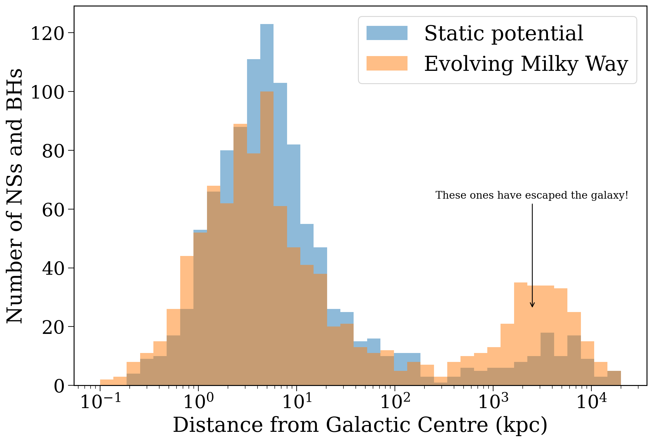
So what do we see? It looks like accounting for the fact that the Milky Way was less massive in its earlier years (we all put on weight in later life, don’t worry MW) means that more compact objects escape the galaxy! The BHs and NSs receive the same kicks in both cases, but the weaker potential in early times can allow more to escape!

Wrap-up

Great work on finishing another tutorial, you’re really plowing through these at a great speed! It seems like you have an appetite for more and don’t you worry, up next we’ll be covering more detailed star formation histories. See you there!

Note

This tutorial was generated from a Jupyter notebook that can be found here.