Changing galactic star formation history models

cogsworth allows you full flexibility in defining your own galactic star formation history (SFH). In addition to the built in galactic star formation models, you can also create your own and use it to generate a population. In this tutorial we’ll walk through how one could do this.

Learning Goals

By the end of this tutorial you should know how to:

• Use a cogsworth star formation history model to sample initial galactic conditions

• Change the star formation history model used in a StarFormationHistory or Population

• Create a custom star formation history model

import cogsworth
import matplotlib.pyplot as plt
import numpy as np
import pandas as pd
import astropy.units as u

# this all just makes plots look nice
%config InlineBackend.figure_format = 'retina'

plt.style.use("dark_background")
plt.rc('font', family='serif')
plt.rcParams['text.usetex'] = False
fs = 24

# update various fontsizes to match
params = {'figure.figsize': (12, 8),
          'legend.fontsize': fs,
          'axes.labelsize': fs,
          'xtick.labelsize': 0.9 * fs,
          'ytick.labelsize': 0.9 * fs,
          'axes.linewidth': 1.1,
          'xtick.major.size': 7,
          'xtick.minor.size': 4,
          'ytick.major.size': 7,
          'ytick.minor.size': 4}
plt.rcParams.update(params)
pd.options.display.max_columns = 999

Star formation histories (SFH)

Each star formation model in cogsworth defines distributions for a couple of things: - Birth times for each system - Initial positions - Metallicities

By default cogsworth will assign initial velocities based on the circular velocity in the chosen galactic potential at the location of the initial position. However, you could in principle also design a class that assigned velocities too.

Let’s start with a very simple star formation history, a burst of star formation at a single time, with a single metallicity, with stars in a cylindrical disc.

We can define this as follows:

s = cogsworth.sfh.BurstUniformDisc(
    t_burst=5 * u.Gyr,
    R_max=15 * u.kpc,
    z_max=2 * u.kpc,
    Z_all=0.02
)

Sampling

Each StarFormationHistory defines the sample() method, which samples initial conditions for a population of systems from the star formation history. By default this will use the built-in modular methods for sampling birth times, initial positions, and metallicities (draw_lookback_times(), draw_radii(), draw_heights(), and get_metallicity()). This allows you override specific functions, but you could also define your own sampling method and do everything all at once.

Let’s start by sampling from the SFH that we just defined above. This just requires us to specify how many points to sample.

s.sample(100_000)

Attributes

BurstUniformDisc inherits from StarFormationHistory and has all of the same attributes. These include:

• x: the initial x positions of each system

• y: the initial y positions of each system

• z: the initial z positions of each system

• v_x: the initial x velocities of each system

• v_y: the initial y velocities of each system

• v_z: the initial z velocities of each system

• tau: the birth times of each system (as a lookback time)

• Z: the metallicities of each system

But you can also get the positions array as .positions or the azimuthal angle as .phi. You can also get the cylindrical radius as .rho. These are all properties that are calculated from the initial positions and velocities.

Let’s take a look at some of these attributes for the population we just sampled.

s.tau, s.rho, s.z

(<Quantity [5., 5., 5., ..., 5., 5., 5.] Gyr>,
 <Quantity [10.63410515,  9.74191915,  0.68491667, ...,  9.10247488,
            10.50453711,  9.22600345] kpc>,
 <Quantity [ 0.08113547, -0.64498773,  1.95347601, ...,  1.67281837,
             0.30101722,  0.32205653] kpc>)

Plotting

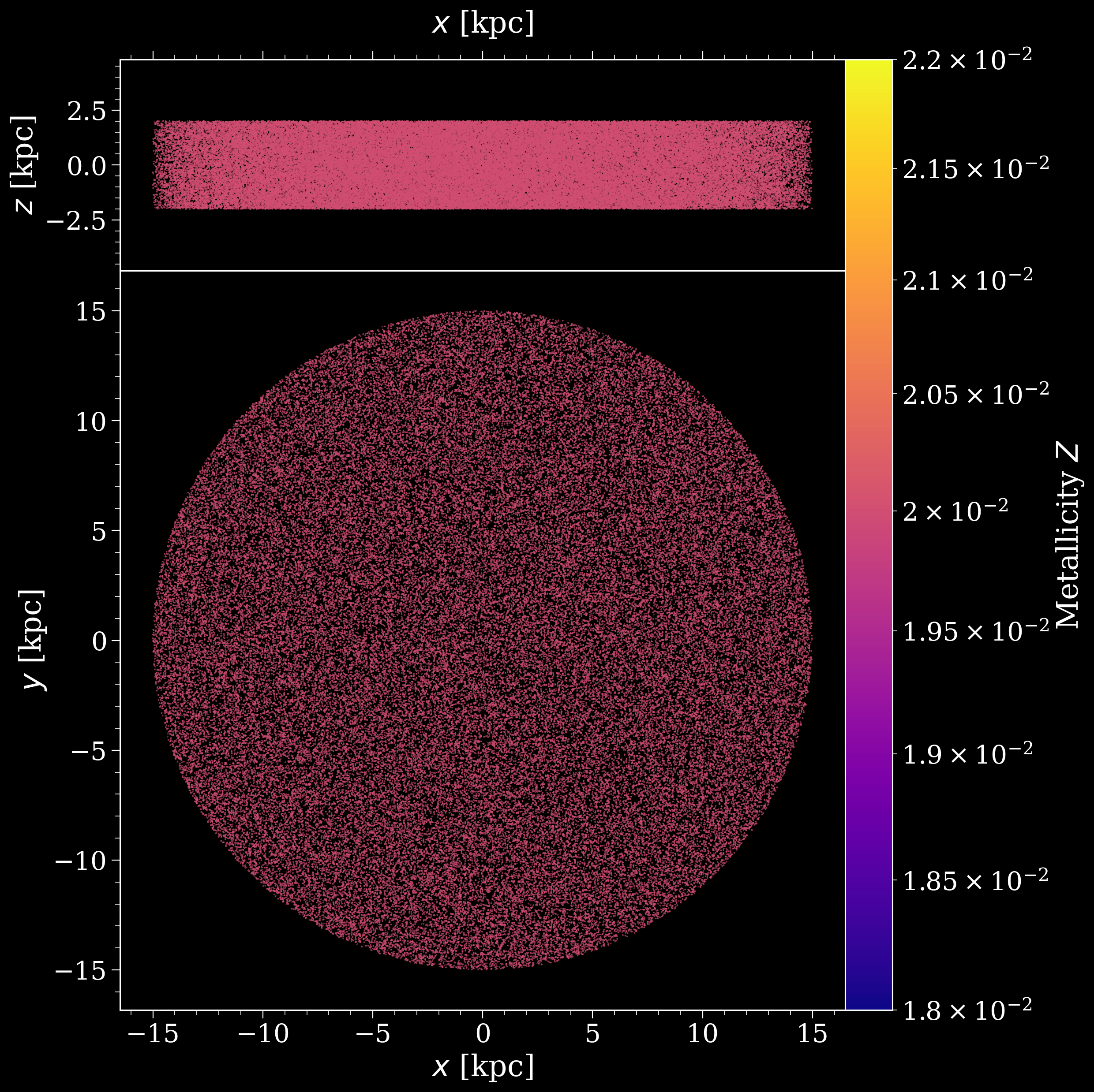
Each SFH also comes with a plotting routine for visualising the spatial distribution of the stars. This is accessed via the plot() method. By default this will show the x-y distribution of the stars and the x-z distribution of the stars, coloured by metallicity. But this is flexible. Let’s try some examples.

fig, axes = s.plot()

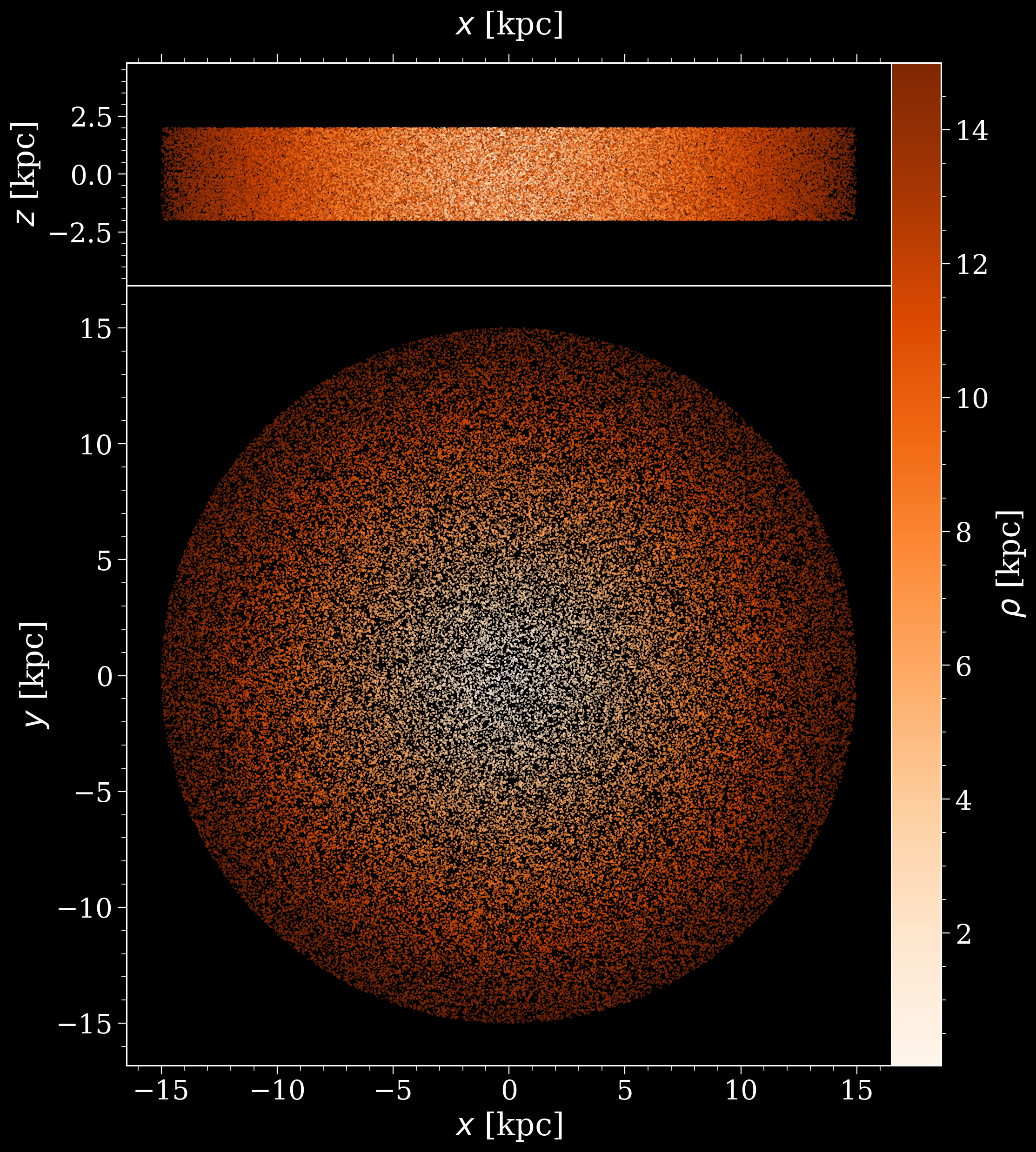
We can also colour by any arbitrary array. Let’s just colour by the radius for now to make it pretty, but in reality the metallicity or lookback time for a more complex SFH may be more interesting.

fig, axes = s.plot(colour_by=s.rho, cbar_label=r'$\rho$ [kpc]', cmap="Oranges")

Composite star formation histories

It’s very common that whatever star formation history you’re considering, there is more than one component to it. For example, you might have multiple discs, a bulge, a halo, or something else. In cogsworth you can define each of these components separately, and then combine them together to make a composite star formation history. This is done by creating multiple StarFormationHistory objects, and then combining them together in a new StarFormationHistory object that takes the individual ones as components.

Combining two SFHs

Let’s start with an example where we combine two different constant uniform disc SFHs together. These SFHs form stars constantly between present day and t_max. We can do this as follows:

small_tall_disc = cogsworth.sfh.ConstantUniformDisc(
    t_burst=5 * u.Gyr,
    R_max=5 * u.kpc,
    z_max=3 * u.kpc,
    Z_all=0.02
)
big_disc = cogsworth.sfh.ConstantUniformDisc(
    t_burst=10 * u.Gyr,
    R_max=15 * u.kpc,
    z_max=1 * u.kpc,
    Z_all=0.001
)

both_discs = small_tall_disc + big_disc
both_discs

<CompositeStarFormationHistory, [not yet sampled], 2 components | ConstantUniformDisc (50%), ConstantUniformDisc (50%)>

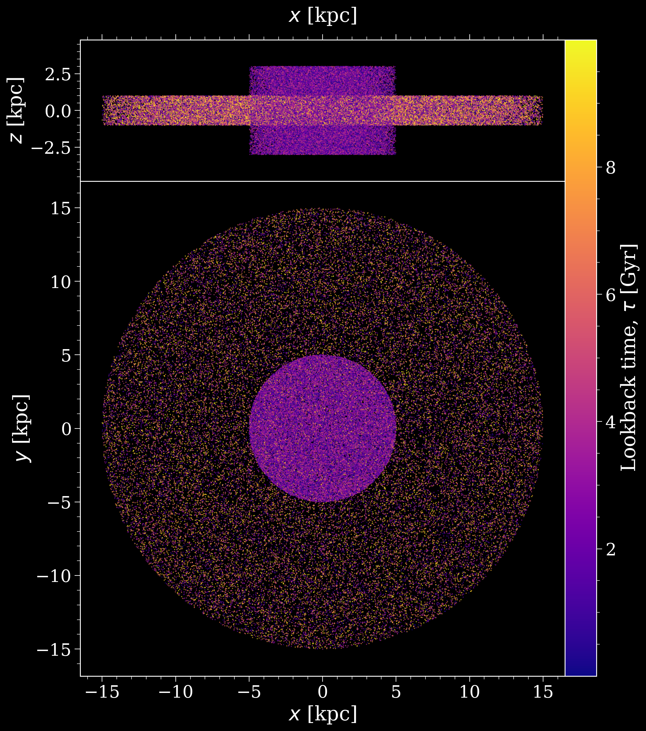
# we can now sample this in the normal way, and plot it as before
both_discs.sample(100_000)
fig, axes = both_discs.plot(colour_by="tau")

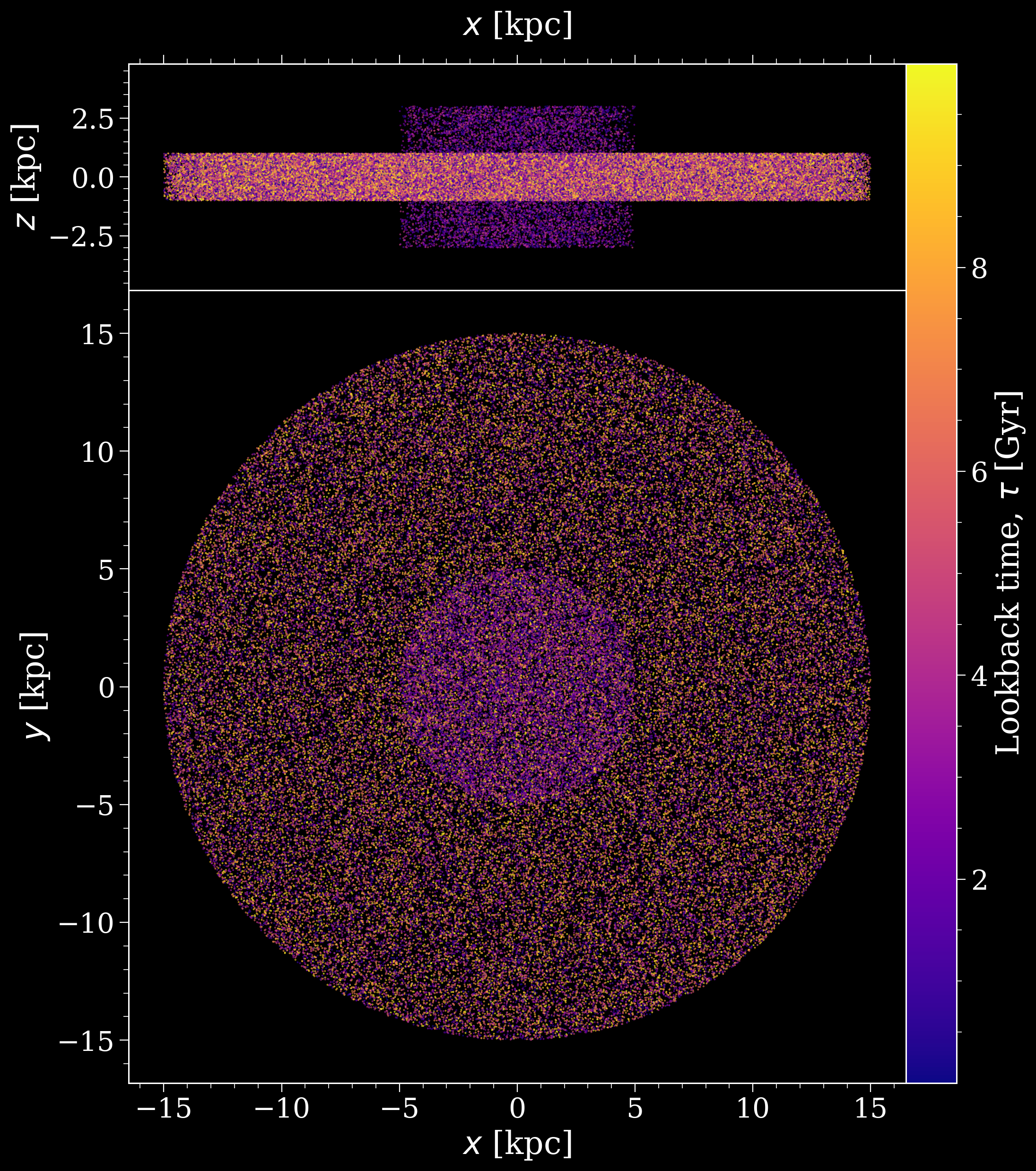
Weighting different components

It’s rarely the case that you want to give each component equal weight. For example, you might want the second disc to have half the mass of the first disc. You can do this by specifying a weight for each component when you combine them together. The weights are relative, so in this example we could give the first disc a weight of 1 and the second disc a weight of 0.5. This is done as follows:

mostly_big_disc = 0.9 * big_disc + 0.1 * small_tall_disc
mostly_big_disc.sample(100_000)
fig, axes = mostly_big_disc.plot(colour_by="tau")

Example: Wagg2022

Before we dive into creating your own custom SFHs, let’s take a look at the default SFH that cogsworth uses, Wagg2022. This model for the Milky Way star formation history was defined in Wagg+2022 and includes the low-$\alpha$ disc, high-$\alpha$ disc and bulge.

w22 = cogsworth.sfh.Wagg2022()
w22.sample(500_000)
w22

<Wagg2022, size=500000, 3 components | LowAlphaDiscWagg2022 (43%), HighAlphaDiscWagg2022 (43%), BulgeWagg2022 (15%)>

fig, axes = w22.plot()

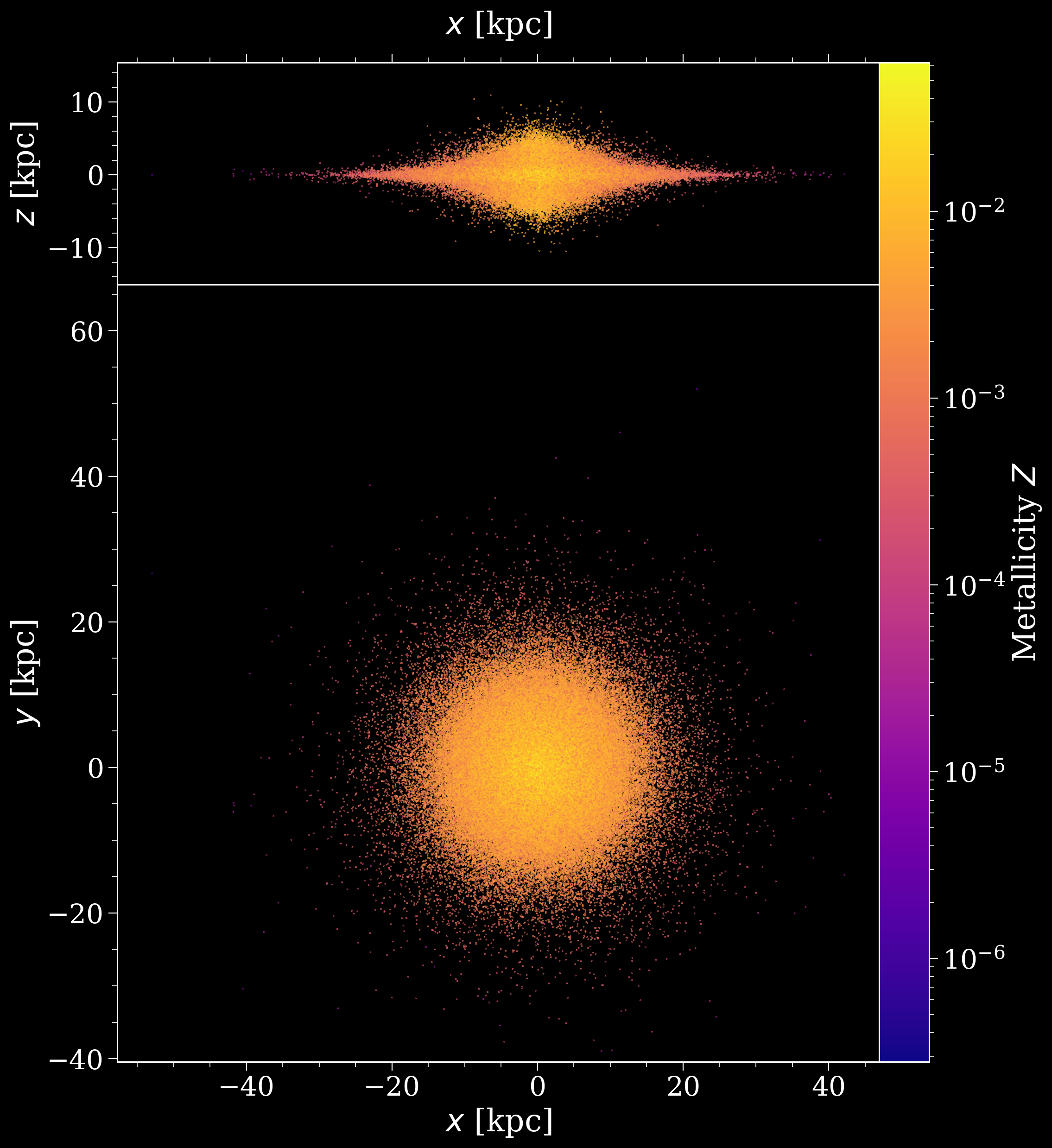
This has called many of this classes methods (e.g. draw_lookback_times, draw_radii etc.) to sample initial conditions (such as tau, rho, Z). You can read more about these exact functions and outputs in the StarFormationHistory docs.

For now let’s take a look at the correlations between radius (w22.rho) and metallicity (w22.Z). The following cell creates a 2D histogram with marginal histograms for each variable.

# create a 2x2 plot with no space between axes
fig, axes = plt.subplots(2, 2, figsize=(15, 15),
                         gridspec_kw={"width_ratios": [5, 1],
                                      "height_ratios": [1, 5]})
fig.subplots_adjust(hspace=0.0, wspace=0.0)

# hide the top right panel
axes[0, 1].axis("off")

# fix the x and y lims
xlims = (1e-2, 50)
ylims = (3e-5, 1e-1)

# add histograms to each axis
axes[0, 0].hist(w22.rho.value, np.geomspace(*xlims, 500))
hexbin = axes[1, 0].hexbin(x=w22.rho.value, y=w22.Z.value, bins="log",
                           xscale="log", yscale="log",
                           extent=np.log10((*xlims, *ylims)))
axes[1, 1].hist(w22.Z.value, np.geomspace(*ylims, 500), orientation="horizontal")

# create an inset axis and add a colourbar
inset_ax = axes[1, 0].inset_axes([0.07, 0.15, 0.6, 0.1])
fig.colorbar(hexbin, cax=inset_ax, orientation="horizontal",
             label="Number of systems")

# set the axes limits, scales and labels
axes[0, 0].set(xlim=xlims, xscale="log")
axes[1, 0].set(xlim=xlims, ylim=ylims, xlabel="Galactocentric radius [kpc]", ylabel="Metallicity")
axes[1, 1].set(ylim=ylims, yscale="log")

# for the marginals hide the ticks and spines
for ax in [axes[0, 0], axes[1, 1]]:
    ax.set(yticks=[], xticks=[])
    ax.spines[:].set_visible(False)

plt.show()

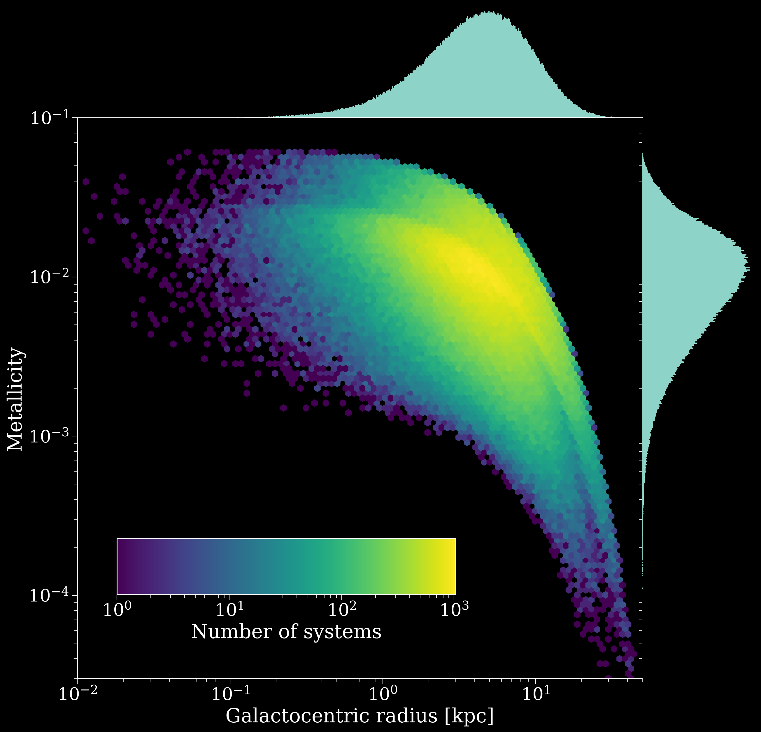
Lovely! So we can see that the highest metallicities are confined to the centre of the galaxy. And all sorts of features in between - do you have any ideas for why there’s a discontinuity in the 2D histogram, what’s that coming from?

The discontinuity comes from…

The discontinuity in the distribution is because this galaxy has multiple components! You can prove this to yourself by only plotting the galaxy for the high-$\alpha$ disc and seeing how things change. Try making the same plot for just the high-$\alpha$ disc and see how the distribution changes. (To do this you can use w22.components[1] to access the high-$\alpha$ disc component of the galaxy, and then plot that).

Why the range of metallicities for each radius, well it depends on when the system was formed. Let’s try colouring by age, and doing some stacked histograms with age bins.

# create a 2x2 plot with no space between axes
fig, axes = plt.subplots(2, 2, figsize=(15, 15),
                         gridspec_kw={"width_ratios": [5, 1],
                                      "height_ratios": [1, 5]})
fig.subplots_adjust(hspace=0.0, wspace=0.0)

# hide the top right panel
axes[0, 1].axis("off")

# fix the x and y lims
xlims = (1e-2, 50)
ylims = (3e-5, 1e-1)

######################
## edited code here ##
######################

time_bins = [(i, i + 3) for i in range(0, 12, 3)] * u.Gyr

# add histograms to each axis
axes[0, 0].hist([w22.rho.value[(w22.tau >= low) & (w22.tau < high)]
                 for low, high in time_bins],
                np.geomspace(*xlims, 500), stacked=True,
                label=[f'{low.value:1.0f}' + r'$< \tau <$' + f'{high.value:1.0f}'
                       for low, high in time_bins])
axes[0, 0].legend(loc="center left", ncol=2, fontsize=0.7*fs)
hexbin = axes[1, 0].hexbin(x=w22.rho.value, y=w22.Z.value, C=w22.tau.value,
                           xscale="log", yscale="log", vmin=0, vmax=12,
                           extent=np.log10((*xlims, *ylims)), cmap="plasma")
axes[1, 1].hist([w22.Z.value[(w22.tau >= low) & (w22.tau < high)]
                 for low, high in time_bins],
                np.geomspace(*ylims, 500), orientation="horizontal", stacked=True)

# create an inset axis and add a colourbar
inset_ax = axes[1, 0].inset_axes([0.07, 0.15, 0.6, 0.1])
fig.colorbar(hexbin, cax=inset_ax, orientation="horizontal",
             label="Lookback time [Gyr]")

######################
## edited code ends ##
######################

# set the axes limits, scales and labels
axes[0, 0].set(xlim=xlims, xscale="log")
axes[1, 0].set(xlim=xlims, ylim=ylims, xlabel="Galactocentric radius [kpc]", ylabel="Metallicity")
axes[1, 1].set(ylim=ylims, yscale="log")

# for the marginals hide the ticks and spines
for ax in [axes[0, 0], axes[1, 1]]:
    ax.set(yticks=[], xticks=[])
    ax.spines[:].set_visible(False)

plt.show()

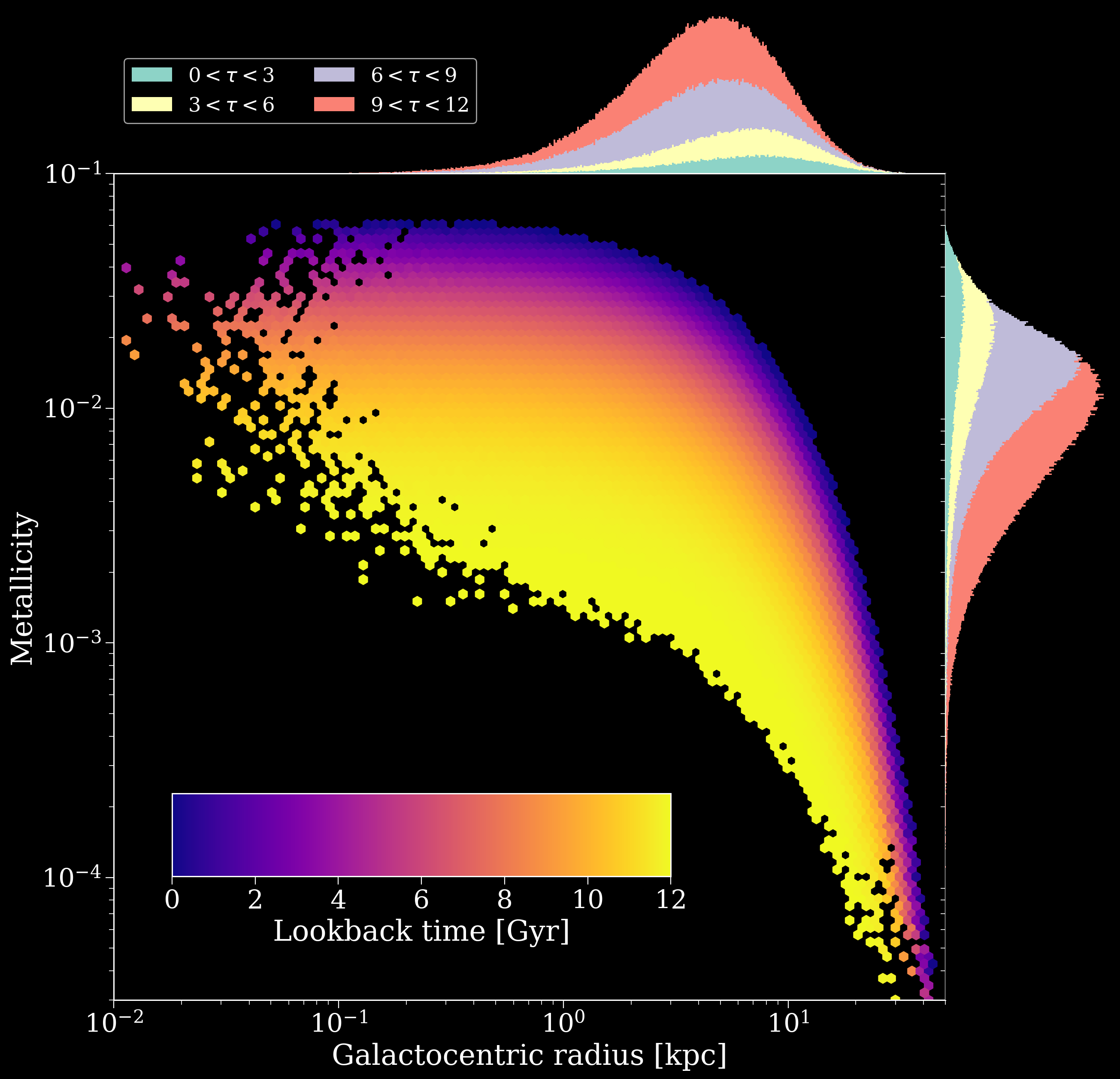
Tip

Lookback time is the time until present day, so lower lookback times mean closer to present day.

Cool right? Given two of radius, age and metallicity we can pinpoint the other in this model. In the marginals you can also see the inside-out growth of the galaxy (more recent times have larger radii) and metal enrichment of the galaxy (more recent times have high metallicity).

Modifying the built-in SFH models

Now let’s say that you want to improve on the built-in cogsworth star formation history models with something more detailed or up-to-date - this should be relatively painless! Let’s consider a couple of scenarios.

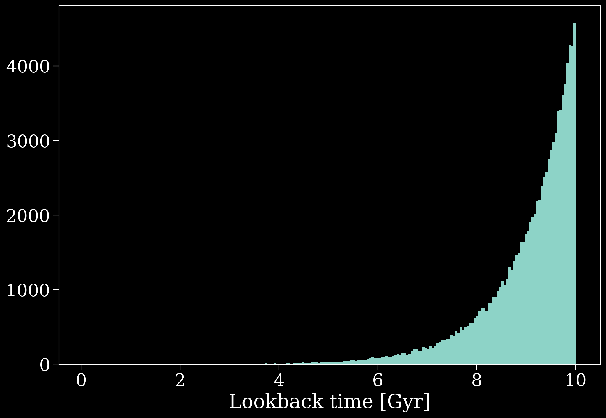
Exponential star formation

Let’s consider that you think perhaps all stars formed in a uniform disc, but that the star formation declines exponentially with time. You could define this as follows:

Hint

Subclasses inherit all of the same functions as their parent classes, so you can overwrite some of the functionality without having to re-invent the wheel. For more info check out the Python documentation on Class Inheritance (it’s less scary than it sounds).

class ExpConstantDisc(cogsworth.sfh.BurstUniformDisc):
    def __init__(self, t_min=0 * u.Gyr, t_max=10 * u.Gyr, *args, **kwargs):
        super().__init__(*args, **kwargs)
        self.t_min = t_min
        self.t_max = t_max

    def draw_lookback_times(self, size):
        U = np.random.random(size)
        return np.log(
            np.exp(self.t_min.to(u.Gyr).value)
            + U
            * (np.exp(self.t_max.to(u.Gyr).value) - np.exp(self.t_min.to(u.Gyr).value))
        ) * u.Gyr

ecd = ExpConstantDisc()
ecd.sample(100_000)

plt.hist(ecd.tau.value, bins="auto");
plt.xlabel("Lookback time [Gyr]")
plt.show()

Fixed metallicity bulge

Perhaps you’re convinced there is only in a fixed low-metallicity population in the bulge, but otherwise you want your model to work exactly as Wagg2022. In this case we can create a subclass based on Wagg2022 that uses a modified bulge component.

# a new class based on BulgeWagg2022
class FixedMetallicityBulge(cogsworth.sfh.BulgeWagg2022):
    # an initialisation function that requires a size and fixed metallicity
    def __init__(self, fixed_Z, *args, **kwargs):
        self.fixed_Z = fixed_Z
        super().__init__(*args, **kwargs)

    # redefine the metallicity function to just return an array of ``fixed_Z``
    def get_metallicity(self):
        return np.repeat(self.fixed_Z, len(self.tau))

# new class based on Wagg2022
class FixedMetallicity(cogsworth.sfh.Wagg2022):
    def __init__(self, fixed_Z, *args, **kwargs):
        self.fixed_Z = fixed_Z
        super().__init__(*args, **kwargs)
        self.components[2] = FixedMetallicityBulge(
            fixed_Z=self.fixed_Z, tsfr=self.tsfr, alpha=self.alpha, Fm=self.Fm,
            gradient=self.gradient, Rnow=self.Rnow, gamma=self.gamma,
            zsun=self.zsun, galaxy_age=self.galaxy_age
        )

Now we can create a SFH based on this just as before.

w22_fixed_Z = FixedMetallicity(fixed_Z=0.02)
w22_fixed_Z.sample(500_000)
w22_fixed_Z.components[2].Z

array([0.02, 0.02, 0.02, ..., 0.02, 0.02, 0.02], shape=(74836,))

Young thick disc

Similarly we could edit the birth time distribution for only the high-$\alpha$ disc of the Wagg2022 model. Let’s imagine you’d made a revolutionary discovery that the high-$\alpha$ disc is actually very young. You could create a new SFH for this as follows:

# a new class based on HighAlphaDiscWagg2022
class YoungDisc(cogsworth.sfh.HighAlphaDiscWagg2022):
    # redefine the lookback time function to just return a uniform distribution in recent years
    def draw_lookback_times(self, size):
        return np.random.uniform(0, 1, size) * u.Gyr

# new class based on Wagg2022
class YoungDiscWagg2022(cogsworth.sfh.Wagg2022):
    def __init__(self, *args, **kwargs):
        super().__init__(*args, **kwargs)
        self.components[1] = YoungDisc(
            tsfr=self.tsfr, alpha=self.alpha, Fm=self.Fm,
            gradient=self.gradient, Rnow=self.Rnow, gamma=self.gamma,
            zsun=self.zsun, galaxy_age=self.galaxy_age
        )

Notice how we can just use the super() definitions of functions in cases where we aren’t changing anything, nice and easy!

w22_young_disc = YoungDiscWagg2022()
w22_young_disc.sample(500_000)

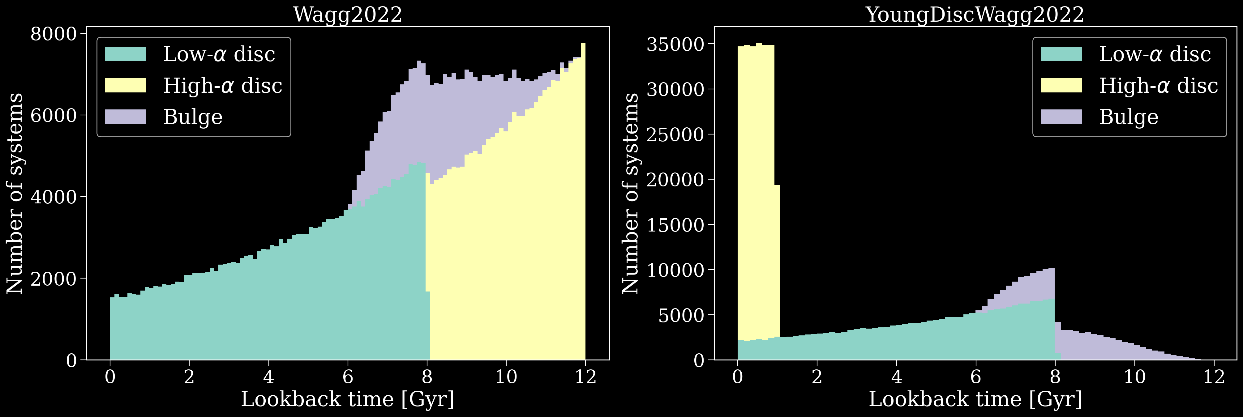
Now let’s compare the age distribution to that of the Wagg2022 model. We can see how, as we defined, all of the bulge systems are now formed in the last billion years, nice!

fig, axes = plt.subplots(1, 2, figsize=(24, 7))

for ax, mod in zip(axes, [w22, w22_young_disc]):
    ax.hist([comp.tau.value for comp in mod.components],
            label=[r'Low-$\alpha$ disc', r'High-$\alpha$ disc', r'Bulge'],
            stacked=True, bins="auto")
    ax.legend()
    ax.set_title(mod.__class__.__name__, fontsize=fs)
    ax.set(xlabel="Lookback time [Gyr]", ylabel="Number of systems")
plt.show()

Defining new SFHs

You also need not restrict yourself to following Wagg2022 or another model, you can define an entire model from scratch. Let’s make a very strange galaxy together!

We create a subclass based off StarFormationHistory to ensure that the same variables are accessible (so that Population can interact with it without confusion), but we can overwrite the majority of the functions.

class TheCube(cogsworth.sfh.StarFormationHistory):
    def sample(self, size):
        self.draw_lookback_times(size)
        self.draw_positions(size)
        self.get_metallicity()

    def draw_lookback_times(self, size):
        self._tau = np.repeat(42, size) * u.Myr

    def draw_positions(self, size):
        self._x = np.random.uniform(-30, 30, size) * u.kpc
        self._y = np.random.uniform(-30, 30, size) * u.kpc
        self._z = np.random.uniform(-30, 30, size) * u.kpc

    def get_metallicity(self):
        nonsense = np.abs(self._x * self._y * self._z)
        self._Z = (nonsense - nonsense.min()) / nonsense.max()

cube = TheCube()
cube.sample(500_000)

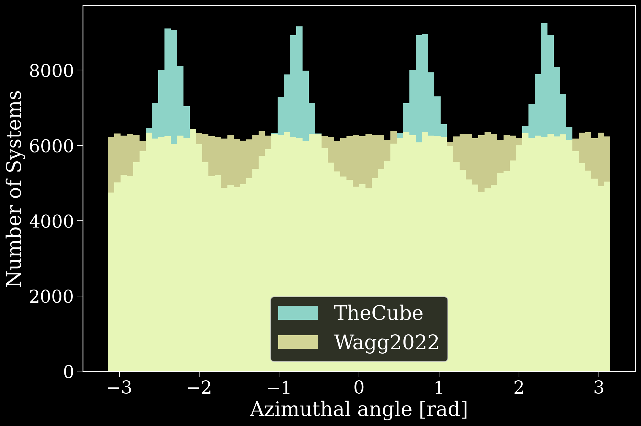
And just like that we’ve defined a rather peculiar galaxy that is shaped like a cube, with everything formed 42 million years ago and some sort of strange metallicity definition. I mean just look at the distribution of phi (azimuthal angle) here - very wacky!

fig, ax = plt.subplots()
ax.hist(cube.phi.value, bins="fd", label="TheCube");
ax.hist(w22.phi.value, bins="fd", alpha=0.8, label="Wagg2022");
ax.set(xlabel="Azimuthal angle [rad]", ylabel="Number of Systems")
ax.legend(loc="lower center")
plt.show()

Using different SFHs in a Population

Okay so we’ve created some new models for galactic star formation histories (some more realistic than others…) - now let’s see how you can plug them into a cogsworth.pop.Population.

Unfortunately, unlike most of cogsworth this is highly technical and can be extremely difficult to pull off…

…nah I’m just kidding, it’s super simple 🙃

p_fixed_Z = cogsworth.pop.Population(
    2000, sfh_model=FixedMetallicity(fixed_Z=0.02),
    use_default_BSE_settings=True
)

Yup, just pass your defined sfh class as sfh_model to the cogsworth.pop.Population and you’re good to go.

Check out how the fixed metallicity population also affects the stars sampled by COSMIC.

p_fixed_Z.sample_initial_binaries()
p_fixed_Z.initial_binaries["metallicity"].values

$[0.03,~0.0231376,~0.0075147735,~\dots,~0.02,~0.02,~0.02] \; \mathrm{}$

And since we went to all of the trouble of making it, let’s use TheCube to evolve a population and see where everything ends up at present day.

p_cube = cogsworth.pop.Population(
    1000, sfh_model=TheCube(),
    use_default_BSE_settings=True
)
p_cube.create_population()

# remove disrupted systems (they go to random locations)
# (you'll learn about masking like this in the next tutorial!)
p_cube = p_cube[~p_cube.disrupted]

Run for 1000 binaries
Sampled 1310 binaries
[1e-02s] Sample initial binaries
[0.2s] Evolve binaries (run COSMIC)

Integrating orbits: 100%|██████████| 1315/1315 [00:00<00:00, 5191.15it/s]

[0.3s] Integrate galactic orbits (run gala)
Overall: 0.5s

fig, axes = plt.subplots(1, 2, figsize=(18, 7), sharey=True)
fig.subplots_adjust(wspace=0.1)

scatter = axes[0].scatter(p_cube.initial_galaxy.x, p_cube.initial_galaxy.y,
                          c=p_cube.initial_galaxy.phi.value, cmap="twilight")

scatter = axes[1].scatter(p_cube.final_pos[:, 0], p_cube.final_pos[:, 1],
                          c=p_cube.initial_galaxy.phi.value, cmap="twilight")
cbar = fig.colorbar(scatter, label=r"$\phi_{\rm init} \, [rad]$", ax=axes, pad=0.0)
cbar.set_ticks([-np.pi, -np.pi / 2, 0, np.pi / 2, np.pi],
               labels=[r'$-\pi$', r'$-\pi / 2$', "0", r'$\pi / 2$', r'$\pi$'])

for ax in axes:
    ax.set(xlabel=r"Galactocentric $x \, [\rm kpc]$",
           xlim=(-40, 40), ylim=(-40, 40))
axes[0].set_ylabel(r"Galactocentric $y \, [\rm kpc]$")

axes[0].annotate("Initial positions", xy=(0.5, 0.95), xycoords="axes fraction",
                 ha="center", va="top", fontsize=0.7*fs)
axes[1].annotate("Final positions", xy=(0.42, 0.96), xycoords="axes fraction",
                 ha="center", va="top", fontsize=0.7*fs, rotation=12)

axes[1].annotate("TheCube...and it's ROTATING!", xy=(0, 1.05), xycoords="axes fraction",
                 ha="center", va="center", fontsize=fs)

plt.show()

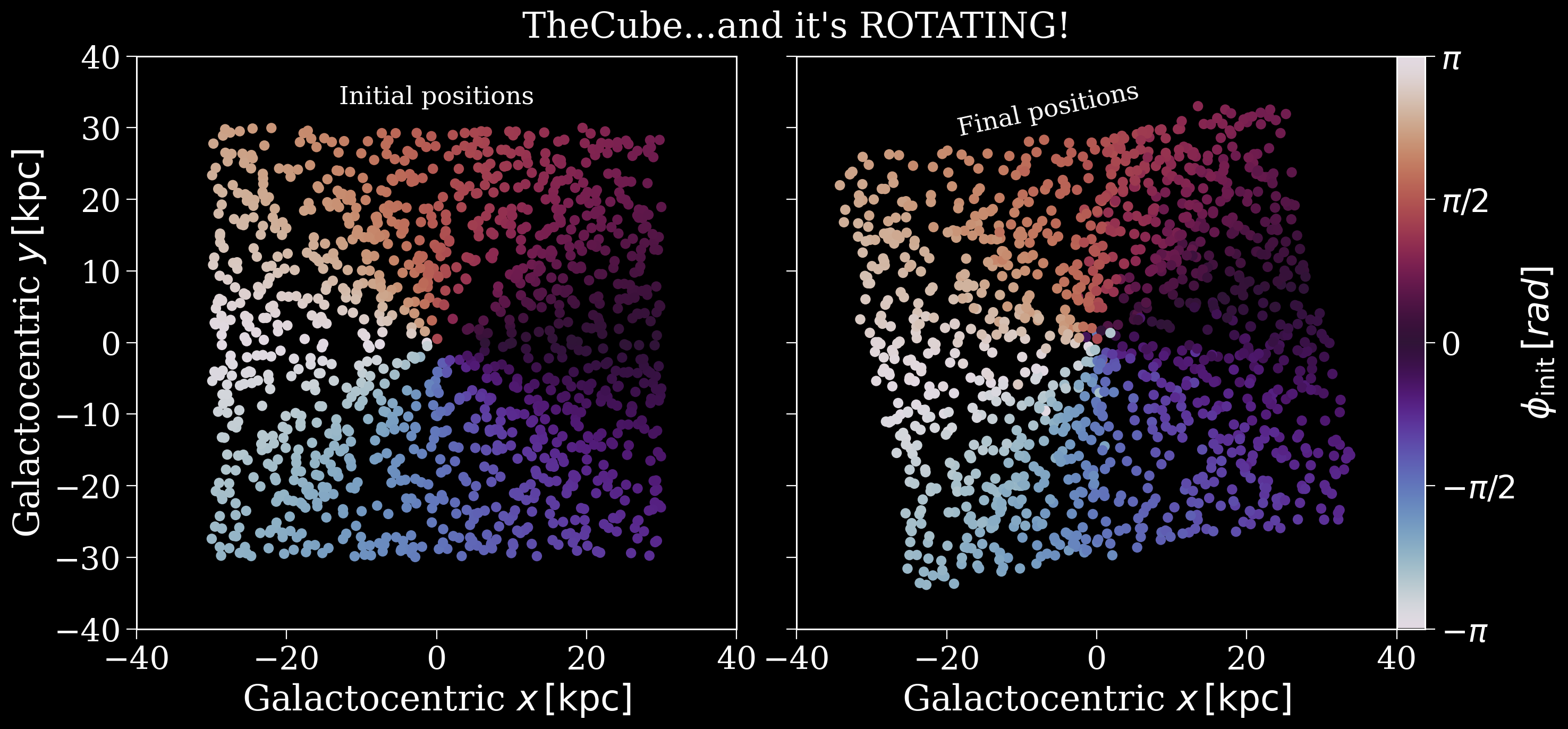
And we have a rotating cube of binaries! Didn’t think that was where this tutorial was going did ya?

Wrap-up

And you’ve made it to the end! Hopefully now you have a good idea of what cogsworth uses by default for its star formation history model, how to make your own models and how to make use of them in a Population.

Keep reading the next tutorials to learn how to mask your population and search for specific subpopulations of interest.

Note

This tutorial was generated from a Jupyter notebook that can be found here.