
Selecting specific subpopulations#
Often when running simulations with cogsworth you will have a specific subpopulation in mind for investigation. It is therefore important to be able to extract this subpopulation from the full population. In this tutorial we’ll go over some basic ways of identifying classes of sources and some more advanced techniques of selecting more unique classes.
Learning Goals#
By the end of this tutorial you should know how to:
Use
determine_final_classes()to identify common source classes in a populationInterface with the
classestable of thePopulationas a shortcut for the above pointDesign a more complex custom mask for a specific subpopulation
For the last point it will be helpful for you to already have a good understanding of the output tables, you can read more in this tutorial.
[1]:
import cogsworth
import matplotlib.pyplot as plt
import numpy as np
import pandas as pd
import astropy.units as u
[2]:
# this all just makes plots look nice
%config InlineBackend.figure_format = 'retina'

plt.rc('font', family='serif')
plt.rcParams['text.usetex'] = False
fs = 24

# update various fontsizes to match
params = {'figure.figsize': (12, 8),
          'legend.fontsize': fs,
          'axes.labelsize': fs,
          'xtick.labelsize': 0.9 * fs,
          'ytick.labelsize': 0.9 * fs,
          'axes.linewidth': 1.1,
          'xtick.major.size': 7,
          'xtick.minor.size': 4,
          'ytick.major.size': 7,
          'ytick.minor.size': 4}
plt.rcParams.update(params)
pd.options.display.max_columns = 999
Indexing Populations#
The Population class is set up so that you can index into it/slice the data convenienting with Python indices or masks. You can either use a list of binary number IDs (or just a single ID) or a boolean mask over all binaries.
Indexing based on bin_num#
Each binary in the Population is assigned a bin_num by COSMIC which will uniquely identify it. These bin_nums are often used as indices for the Pandas tables and will always be included as a column in the table. You can use these to index a Population like this
[3]:
p = cogsworth.pop.Population(20, use_default_BSE_settings=True)
p.create_population(with_timing=False)
p
[3]:
<Population - 25 evolved systems - galactic_potential=MilkyWayPotential, sfh_model=Wagg2022>
[4]:
# you can list out the bin_nums like this
p.bin_nums
[4]:
array([ 0,  1,  2,  3,  4,  5,  6,  7,  8,  9, 10, 11, 12, 13, 14, 15, 16,
       17, 18, 19, 20, 21, 22, 23, 24])
[5]:
p_small = p[[4, 2]]
p_small
[5]:
<Population - 2 evolved systems - galactic_potential=MilkyWayPotential, sfh_model=Wagg2022>
We can also do usual slicing things, like getting every other binary between 2 and 10
[6]:
p_every_other = p[2:10:2]
p_every_other.bin_nums
[6]:
array([2, 4, 6, 8])
Indexing based on a mask#
Alternatively, if you have some condition that every binary needs to meet you can use this to index your population rather directly target certain bin_nums. This can be useful for creating complicated conditions as we’ll see later in the tutorial.
[7]:
mask = np.repeat(False, len(p))
mask[:5] = True
print(mask)
p_masked = p[mask]
p_masked
[ True  True  True  True  True False False False False False False False
 False False False False False False False False False False False False
 False]
[7]:
<Population - 5 evolved systems - galactic_potential=MilkyWayPotential, sfh_model=Wagg2022>
Identifying common classes#
Now let’s consider the determine_final_classes() function. As one might expect from the name, this takes the final state of the population and determines the classes of each source. As input this requires most of the usual population outputs and can be used manually, but it is much easier to access it through a Population.
Let’s try it out! We can first make a tiny population and tell COSMIC to prioritise sampling binaries that will have a component that’s a black hole or a neutron star
[8]:
p = cogsworth.pop.Population(100, final_kstar1=[13, 14],
                             use_default_BSE_settings=True)
p.create_population()
Run for 100 binaries
Sampled 100 binaries
[9e-03s] Sample initial binaries
[0.2s] Evolve binaries (run COSMIC)
Integrating orbits: 100%|██████████| 107/107 [00:00<00:00, 1319.41it/s]
[0.3s] Integrate galactic orbits (run gala)
Overall: 0.5s
Now to get the classes for each source we just need to access p.classes
[9]:
p.classes
[9]:
| dco | co-1 | co-2 | xrb | walkaway-t-1 | walkaway-t-2 | runaway-t-1 | runaway-t-2 | walkaway-o-1 | walkaway-o-2 | runaway-o-1 | runaway-o-2 | widow-1 | widow-2 | stellar-merger-co-1 | stellar-merger-co-2 | |
|---|---|---|---|---|---|---|---|---|---|---|---|---|---|---|---|---|
| 0 | False | False | False | False | False | False | False | False | False | False | False | False | False | False | False | False |
| 1 | False | False | False | False | False | False | False | False | False | False | False | False | False | False | False | False |
| 2 | False | False | False | False | False | False | False | False | False | False | False | False | False | False | False | False |
| 3 | False | False | False | False | False | False | False | False | False | False | False | False | False | False | False | False |
| 4 | False | False | False | False | False | False | False | False | False | False | False | False | False | False | False | True |
| ... | ... | ... | ... | ... | ... | ... | ... | ... | ... | ... | ... | ... | ... | ... | ... | ... |
| 95 | False | False | False | False | False | False | False | False | False | False | False | False | False | False | False | False |
| 96 | False | False | False | False | False | False | False | False | False | False | False | False | False | False | False | False |
| 97 | False | False | False | False | False | False | False | False | False | False | False | False | False | False | False | False |
| 98 | False | False | False | False | False | False | False | False | False | False | False | False | False | False | False | False |
| 99 | False | True | False | False | False | False | False | False | False | False | False | False | False | False | False | False |
100 rows × 16 columns
This gives us a huge table of booleans, which indicate whether a source is a part of a particular class. Each source can therefore have multiple classes (e.g. all dcos will also have co-1 and co-2).
We can summarise this as totals by running the following
[10]:
p.classes.sum()
[10]:
dco                     1
co-1                    8
co-2                    2
xrb                     0
walkaway-t-1            0
walkaway-t-2            0
runaway-t-1             0
runaway-t-2             0
walkaway-o-1            0
walkaway-o-2            0
runaway-o-1             0
runaway-o-2             0
widow-1                 0
widow-2                 0
stellar-merger-co-1    21
stellar-merger-co-2    14
dtype: int64
Available classes#
Don’t worry if those names seem arcane, you can always get a list of the current supported classes with list_classes() :)
[11]:
cogsworth.classify.list_classes()
Any class with a suffix '-1' or '-2' applies to only the primary or secondary
Available classes
-----------------
Theory Runaway (runaway-t)
    Any star from a disrupted binary that has an instantaneous velocity > 30 km/s in the frame of the binary

Observation runaway (runaway-o)
    Any star from a disrupted binary that is moving with a Galactocentric velocity > 30km/s relative to the local circular velocity at its location

Theory Runaway (walkaway-t)
    Any star from a disrupted binary that has an instantaneous velocity < 30 km/s in the frame of the binary

Observation walkaway (walkaway-o)
    Any star from a disrupted binary that is moving with a Galactocentric velocity < 30km/s relative to the local circular velocity at its location

Widowed Star (widow)
    Any star, or binary containing a star, that is/was a companion to a compact object

X-ray binary (xrb)
    Any binary with a star that is a companion to a compact object

Compact object (co)
    Any compact object or binary containing a compact object

Compact object from merger (stellar-merger-co)
    Any compact object resulting from a stellar merger

Double compact object (dco)
    Any bound binary of two compact objects

Single degenerate type Ia (sdIa)
    Any disrupted binary that contains a massless remnant that was once a white dwarf
Selecting only compact objects#
Okay as an example, let’s select just the sources that have a primary that is a compact object. Each column of the classes table is a boolean array that we can apply as a mask to the population.
[12]:
p.classes["co-1"].values
[12]:
array([False, False, False, False, False, False, False,  True, False,
       False, False, False, False, False, False, False, False, False,
       False, False, False, False, False,  True, False, False, False,
       False, False, False, False, False, False, False, False, False,
       False, False, False, False, False, False,  True, False, False,
       False, False, False, False, False, False, False, False,  True,
       False, False, False,  True, False, False, False, False, False,
       False, False, False, False,  True, False, False, False, False,
       False, False, False, False, False, False, False, False, False,
       False, False, False, False, False, False, False, False,  True,
       False, False, False, False, False, False, False, False, False,
        True])
[13]:
co1_pop = p[p.classes["co-1"]]
Let’s check out the final_bpp table to confirm that we’ve selected the right things.
[14]:
co1_pop.final_bpp
[14]:
| tphys | mass_1 | mass_2 | kstar_1 | kstar_2 | sep | porb | ecc | RRLO_1 | RRLO_2 | evol_type | aj_1 | aj_2 | tms_1 | tms_2 | massc_he_layer_1 | massc_he_layer_2 | massc_co_layer_1 | massc_co_layer_2 | rad_1 | rad_2 | mass0_1 | mass0_2 | lum_1 | lum_2 | teff_1 | teff_2 | radc_1 | radc_2 | menv_1 | menv_2 | renv_1 | renv_2 | omega_spin_1 | omega_spin_2 | B_1 | B_2 | bacc_1 | bacc_2 | tacc_1 | tacc_2 | epoch_1 | epoch_2 | bhspin_1 | bhspin_2 | bin_num | metallicity | |
|---|---|---|---|---|---|---|---|---|---|---|---|---|---|---|---|---|---|---|---|---|---|---|---|---|---|---|---|---|---|---|---|---|---|---|---|---|---|---|---|---|---|---|---|---|---|---|---|
| 7 | 7661.636671 | 2.608801 | 0.904320 | 13 | 11 | -1.000000 | -1.000000 | -1.00000 | 1.000000e-04 | 1.000000e-04 | 10 | 7650.683887 | 7556.969872 | 1.000000e+10 | 1.000000e+10 | 0.0 | 0.0 | 0.0 | 0.0 | 0.000014 | 0.009130 | 17.806158 | 0.904320 | 6.495983e-10 | 4.779652e-05 | 7822.882631 | 5045.293620 | 0.000014 | 0.009130 | 1.000000e-10 | 1.000000e-10 | 1.000000e-10 | 1.000000e-10 | 2.016194e+06 | 6.317276e-06 | 1.049189e+12 | 0.000000e+00 | 0.0 | 0.0 | 0.0 | 0.0 | 10.952784 | 104.666799 | 0.0 | 0.0 | 7 | 0.012829 |
| 23 | 1380.501861 | 1.277584 | 2.106171 | 13 | 13 | -1.000000 | -1.000000 | -1.00000 | 1.000000e-04 | 1.000000e-04 | 10 | 1367.543958 | 1365.699534 | 1.000000e+10 | 1.000000e+10 | 0.0 | 0.0 | 0.0 | 0.0 | 0.000014 | 0.000014 | 3.100954 | 6.111151 | 1.260167e-08 | 1.766284e-08 | 16417.712758 | 17863.670575 | 0.000014 | 0.000014 | 1.000000e-10 | 1.000000e-10 | 1.000000e-10 | 1.000000e-10 | 6.735002e+06 | 1.037633e+07 | 3.192609e+12 | 2.072515e+12 | 0.0 | 0.0 | 0.0 | 0.0 | 12.957903 | 14.802326 | 0.0 | 0.0 | 23 | 0.030000 |
| 42 | 4720.876220 | 1.656706 | 0.730577 | 13 | 11 | -1.000000 | -1.000000 | -1.00000 | 1.000000e-04 | 1.000000e-04 | 10 | 4712.134008 | 4423.993442 | 1.000000e+10 | 1.000000e+10 | 0.0 | 0.0 | 0.0 | 0.0 | 0.000014 | 0.011125 | 4.883718 | 0.730577 | 1.263250e-09 | 7.761081e-05 | 9237.998743 | 5159.297994 | 0.000014 | 0.011125 | 1.000000e-10 | 1.000000e-10 | 1.000000e-10 | 1.000000e-10 | 6.509123e+06 | 5.265949e-06 | 8.038951e+11 | 0.000000e+00 | 0.0 | 0.0 | 0.0 | 0.0 | 8.742212 | 296.882778 | 0.0 | 0.0 | 42 | 0.015142 |
| 53 | 8049.453428 | 1.277584 | 0.614300 | 13 | 11 | -1.000000 | -1.000000 | -1.00000 | 1.000000e-04 | 1.000000e-04 | 10 | 8025.253678 | 6298.889235 | 1.000000e+10 | 1.000000e+10 | 0.0 | 0.0 | 0.0 | 0.0 | 0.000014 | 0.012587 | 10.688992 | 0.614300 | 3.659260e-10 | 3.743586e-05 | 6777.256392 | 4042.345187 | 0.000014 | 0.012587 | 1.000000e-10 | 1.000000e-10 | 1.000000e-10 | 1.000000e-10 | 1.152194e+06 | 4.892916e-06 | 1.626998e+12 | 0.000000e+00 | 0.0 | 0.0 | 0.0 | 0.0 | 24.199750 | 1750.564193 | 0.0 | 0.0 | 53 | 0.010702 |
| 57 | 9581.980933 | 1.277584 | 0.856462 | 13 | 11 | -1.000000 | -1.000000 | -1.00000 | 1.000000e-04 | 1.000000e-04 | 10 | 9540.756241 | 9454.244926 | 1.000000e+10 | 1.000000e+10 | 0.0 | 0.0 | 0.0 | 0.0 | 0.000014 | 0.009668 | 8.161255 | 0.856462 | 2.589079e-10 | 1.765915e-05 | 6215.726554 | 3822.529655 | 0.000014 | 0.009668 | 1.000000e-10 | 1.000000e-10 | 1.000000e-10 | 1.000000e-10 | 3.204501e+06 | 5.948781e-06 | 3.599979e+11 | 0.000000e+00 | 0.0 | 0.0 | 0.0 | 0.0 | 41.224692 | 127.736007 | 0.0 | 0.0 | 57 | 0.004534 |
| 67 | 10961.876476 | 18.886369 | 12.717184 | 14 | 14 | 2439.861274 | 2484.573845 | 0.25488 | 1.065061e-07 | 8.590900e-08 | 10 | 10957.576293 | 10956.116541 | 1.000000e+10 | 1.000000e+10 | 0.0 | 0.0 | 0.0 | 0.0 | 0.000080 | 0.000054 | 17.563047 | 14.068570 | 1.000000e-10 | 1.000000e-10 | 2048.860791 | 2496.842844 | 0.000080 | 0.000054 | 1.000000e-10 | 1.000000e-10 | 1.000000e-10 | 1.000000e-10 | 1.200841e+11 | 2.000000e+08 | 0.000000e+00 | 0.000000e+00 | 0.0 | 0.0 | 0.0 | 0.0 | 4.300184 | 5.759935 | 0.0 | 0.0 | 67 | 0.004345 |
| 89 | 6787.641441 | 1.277584 | 0.916640 | 13 | 11 | -1.000000 | -1.000000 | -1.00000 | 1.000000e-04 | 1.000000e-04 | 10 | 6761.568587 | 6692.616434 | 1.000000e+10 | 1.000000e+10 | 0.0 | 0.0 | 0.0 | 0.0 | 0.000014 | 0.008992 | 10.214439 | 0.916640 | 5.154849e-10 | 5.315164e-05 | 7383.453969 | 5220.602738 | 0.000014 | 0.008992 | 1.000000e-10 | 1.000000e-10 | 1.000000e-10 | 1.000000e-10 | 1.309188e+06 | 6.424946e-06 | 2.000148e+12 | 0.000000e+00 | 0.0 | 0.0 | 0.0 | 0.0 | 26.072854 | 95.025007 | 0.0 | 0.0 | 89 | 0.011302 |
| 99 | 8141.486444 | 1.277584 | 0.649690 | 13 | 11 | -1.000000 | -1.000000 | -1.00000 | 1.000000e-04 | 1.000000e-04 | 10 | 8118.976163 | 7446.364621 | 1.000000e+10 | 1.000000e+10 | 0.0 | 0.0 | 0.0 | 0.0 | 0.000014 | 0.012125 | 11.051045 | 0.649690 | 3.575265e-10 | 3.429836e-05 | 6738.025766 | 4029.410958 | 0.000014 | 0.012125 | 1.000000e-10 | 1.000000e-10 | 1.000000e-10 | 1.000000e-10 | 7.241473e+05 | 4.985277e-06 | 2.567682e+12 | 0.000000e+00 | 0.0 | 0.0 | 0.0 | 0.0 | 22.510281 | 695.121823 | 0.0 | 0.0 | 99 | 0.012247 |
You can see that the kstar_1 column is always either 13 (neutron star) or 14 (black hole), nice!
Custom subpopulations#
Now I have not likely managed to anticipate your exact use case and class, but never fear, you can create a custom mask based on all sorts of aspects of a Population!
Conditioning on the final state#
Let’s say that we now want any system that has disrupted and has a compact object as the secondary. First we can use the helper mask .disrupted, which is a boolean for each binary which flags whether it was disrupted by a supernova or not (it works this out based on the bpp and kick_info tables), then we combine that with the .classes table.
[15]:
custom_mask = p.disrupted & p.classes["co-2"]
custom_pop = p[custom_mask]
custom_pop.final_bpp
[15]:
| tphys | mass_1 | mass_2 | kstar_1 | kstar_2 | sep | porb | ecc | RRLO_1 | RRLO_2 | evol_type | aj_1 | aj_2 | tms_1 | tms_2 | massc_he_layer_1 | massc_he_layer_2 | massc_co_layer_1 | massc_co_layer_2 | rad_1 | rad_2 | mass0_1 | mass0_2 | lum_1 | lum_2 | teff_1 | teff_2 | radc_1 | radc_2 | menv_1 | menv_2 | renv_1 | renv_2 | omega_spin_1 | omega_spin_2 | B_1 | B_2 | bacc_1 | bacc_2 | tacc_1 | tacc_2 | epoch_1 | epoch_2 | bhspin_1 | bhspin_2 | bin_num | metallicity | |
|---|---|---|---|---|---|---|---|---|---|---|---|---|---|---|---|---|---|---|---|---|---|---|---|---|---|---|---|---|---|---|---|---|---|---|---|---|---|---|---|---|---|---|---|---|---|---|---|
| 23 | 1380.501861 | 1.277584 | 2.106171 | 13 | 13 | -1.0 | -1.0 | -1.0 | 0.0001 | 0.0001 | 10 | 1367.543958 | 1365.699534 | 1.000000e+10 | 1.000000e+10 | 0.0 | 0.0 | 0.0 | 0.0 | 0.000014 | 0.000014 | 3.100954 | 6.111151 | 1.260167e-08 | 1.766284e-08 | 16417.712758 | 17863.670575 | 0.000014 | 0.000014 | 1.000000e-10 | 1.000000e-10 | 1.000000e-10 | 1.000000e-10 | 6.735002e+06 | 1.037633e+07 | 3.192609e+12 | 2.072515e+12 | 0.0 | 0.0 | 0.0 | 0.0 | 12.957903 | 14.802326 | 0.0 | 0.0 | 23 | 0.03 |
Okay let’s be more specific, we also want it to be specifically a neutron star of at least 1.2 solar masses - you can just keep stringing together the conditions!
[16]:
custom_mask = p.disrupted & p.classes["co-2"]\
    & (p.final_bpp["kstar_2"] == 13) & (p.final_bpp["mass_2"] > 1.2)
custom_pop = p[custom_mask]
custom_pop.final_bpp
[16]:
| tphys | mass_1 | mass_2 | kstar_1 | kstar_2 | sep | porb | ecc | RRLO_1 | RRLO_2 | evol_type | aj_1 | aj_2 | tms_1 | tms_2 | massc_he_layer_1 | massc_he_layer_2 | massc_co_layer_1 | massc_co_layer_2 | rad_1 | rad_2 | mass0_1 | mass0_2 | lum_1 | lum_2 | teff_1 | teff_2 | radc_1 | radc_2 | menv_1 | menv_2 | renv_1 | renv_2 | omega_spin_1 | omega_spin_2 | B_1 | B_2 | bacc_1 | bacc_2 | tacc_1 | tacc_2 | epoch_1 | epoch_2 | bhspin_1 | bhspin_2 | bin_num | metallicity | |
|---|---|---|---|---|---|---|---|---|---|---|---|---|---|---|---|---|---|---|---|---|---|---|---|---|---|---|---|---|---|---|---|---|---|---|---|---|---|---|---|---|---|---|---|---|---|---|---|
| 23 | 1380.501861 | 1.277584 | 2.106171 | 13 | 13 | -1.0 | -1.0 | -1.0 | 0.0001 | 0.0001 | 10 | 1367.543958 | 1365.699534 | 1.000000e+10 | 1.000000e+10 | 0.0 | 0.0 | 0.0 | 0.0 | 0.000014 | 0.000014 | 3.100954 | 6.111151 | 1.260167e-08 | 1.766284e-08 | 16417.712758 | 17863.670575 | 0.000014 | 0.000014 | 1.000000e-10 | 1.000000e-10 | 1.000000e-10 | 1.000000e-10 | 6.735002e+06 | 1.037633e+07 | 3.192609e+12 | 2.072515e+12 | 0.0 | 0.0 | 0.0 | 0.0 | 12.957903 | 14.802326 | 0.0 | 0.0 | 23 | 0.03 |
Conditioning on evolutionary history#
Or we could even condition on the evolutionary history rather than just the final state. Let’s grab any binary that at any point in its evolution reversed its mass ratio whilst both components were still stars.
Since the evolutionary history table has multiple entries for each binary we need to identify things based on the binary number rather than a simple mask (since the table has a different length than the number of binaries).
[17]:
# get every row of evolutionary history matching condition
rev_mr_rows = p.bpp[(p.bpp["mass_2"] > p.bpp["mass_1"])
                    & (p.bpp["kstar_1"] < 7)
                    & (p.bpp["kstar_2"] < 7)]

# get unique binary numbers matching mask
rev_mr_bin_nums = rev_mr_rows["bin_num"].unique()

# mask the population
custom_pop = p[rev_mr_bin_nums]
Let’s look at the evolution history of the first binary in this bunch to confirm we masked the right things
[18]:
custom_pop.bpp.loc[custom_pop.bin_nums[0]]
[18]:
| tphys | mass_1 | mass_2 | kstar_1 | kstar_2 | sep | porb | ecc | RRLO_1 | RRLO_2 | evol_type | aj_1 | aj_2 | tms_1 | tms_2 | massc_he_layer_1 | massc_he_layer_2 | massc_co_layer_1 | massc_co_layer_2 | rad_1 | rad_2 | mass0_1 | mass0_2 | lum_1 | lum_2 | teff_1 | teff_2 | radc_1 | radc_2 | menv_1 | menv_2 | renv_1 | renv_2 | omega_spin_1 | omega_spin_2 | B_1 | B_2 | bacc_1 | bacc_2 | tacc_1 | tacc_2 | epoch_1 | epoch_2 | bhspin_1 | bhspin_2 | bin_num | |
|---|---|---|---|---|---|---|---|---|---|---|---|---|---|---|---|---|---|---|---|---|---|---|---|---|---|---|---|---|---|---|---|---|---|---|---|---|---|---|---|---|---|---|---|---|---|---|
| 13 | 0.000000 | 3.481164 | 2.861476 | 1 | 1 | 4027.858752 | 11763.823157 | 0.672578 | 0.003874 | 0.003804 | 1 | 0.000000 | 0.000000 | 2.451667e+02 | 4.062730e+02 | 0.000000 | 0.000000 | 0.000000 | 0.000000 | 2.023445 | 1.816317 | 3.481164 | 2.861476 | 152.865079 | 73.612413 | 14331.807889 | 12601.188756 | 0.000000 | 0.000000 | 1.000000e-10 | 1.000000e-10 | 1.000000e-10 | 1.000000e-10 | 6.638707e+03 | 7535.984211 | 0.0 | 0.0 | 0.0 | 0.0 | 0.0 | 0.0 | 0.000000 | 0.000000 | 0.0 | 0.0 | 13 |
| 13 | 245.226203 | 3.480589 | 2.861464 | 2 | 1 | 4028.231208 | 11765.998882 | 0.672578 | 0.009015 | 0.005538 | 2 | 245.268781 | 245.226330 | 2.452688e+02 | 4.062773e+02 | 0.514852 | 0.000000 | 0.000000 | 0.000000 | 4.708092 | 2.644675 | 3.480589 | 2.861464 | 399.630806 | 103.520455 | 11947.083526 | 11372.081357 | 0.114089 | 0.000000 | 1.000000e-10 | 1.000000e-10 | 1.000000e-10 | 1.000000e-10 | 1.436835e+03 | 3554.386816 | 0.0 | 0.0 | 0.0 | 0.0 | 0.0 | 0.0 | -0.042578 | -0.000127 | 0.0 | 0.0 | 13 |
| 13 | 246.580752 | 3.480346 | 2.861464 | 3 | 1 | 4028.385461 | 11766.900199 | 0.672578 | 0.039418 | 0.005554 | 2 | 246.666693 | 246.580872 | 2.453120e+02 | 4.062773e+02 | 0.525700 | 0.000000 | 0.000000 | 0.000000 | 20.587915 | 2.652688 | 3.480346 | 2.861464 | 234.177177 | 103.767869 | 4998.613610 | 11361.672157 | 0.116678 | 0.000000 | 1.477352e+00 | 1.000000e-10 | 1.330644e+01 | 1.000000e-10 | 5.654082e+01 | 3532.947331 | 0.0 | 0.0 | 0.0 | 0.0 | 0.0 | 0.0 | -0.085941 | -0.000121 | 0.0 | 0.0 | 13 |
| 13 | 247.658525 | 3.479363 | 2.861465 | 4 | 1 | 4029.006699 | 11770.533491 | 0.672578 | 0.102499 | 0.005566 | 2 | 247.744466 | 247.658443 | 2.453120e+02 | 4.062770e+02 | 0.540507 | 0.000000 | 0.000000 | 0.000000 | 53.539459 | 2.659116 | 3.480346 | 2.861465 | 984.314550 | 103.965685 | 4438.294295 | 11353.335258 | 0.120138 | 0.000000 | 2.938856e+00 | 1.000000e-10 | 5.341932e+01 | 1.000000e-10 | 8.386691e+00 | 3515.890364 | 0.0 | 0.0 | 0.0 | 0.0 | 0.0 | 0.0 | -0.085941 | 0.000082 | 0.0 | 0.0 | 13 |
| 13 | 297.232135 | 3.447137 | 2.861485 | 5 | 1 | 4049.502542 | 11890.699478 | 0.672576 | 0.074373 | 0.006274 | 2 | 297.318077 | 297.227091 | 2.453120e+02 | 4.062695e+02 | 0.370072 | 0.000000 | 0.438556 | 0.000000 | 38.965191 | 3.018969 | 3.480346 | 2.861485 | 623.317116 | 113.911433 | 4640.966898 | 10901.395434 | 0.173164 | 0.000000 | 2.638510e+00 | 1.000000e-10 | 3.879203e+01 | 1.000000e-10 | 1.631723e+01 | 2727.738484 | 0.0 | 0.0 | 0.0 | 0.0 | 0.0 | 0.0 | -0.085941 | 0.005045 | 0.0 | 0.0 | 13 |
| 13 | 299.235993 | 3.409894 | 2.862094 | 6 | 1 | 3941.774208 | 11452.681254 | 0.661343 | 0.592249 | 0.006253 | 2 | 299.321934 | 299.063476 | 2.453120e+02 | 4.060421e+02 | 0.000000 | 0.000000 | 0.803796 | 0.000000 | 311.630385 | 3.037302 | 3.480346 | 2.862094 | 12891.831768 | 114.446080 | 3499.680279 | 10881.175857 | 0.051337 | 0.000000 | 2.606097e+00 | 1.000000e-10 | 3.115790e+02 | 1.000000e-10 | 6.158425e-01 | 2697.771079 | 0.0 | 0.0 | 0.0 | 0.0 | 0.0 | 0.0 | -0.085941 | 0.172517 | 0.0 | 0.0 | 13 |
| 13 | 299.797965 | 1.713028 | 3.204495 | 6 | 1 | 2025.936057 | 4765.819516 | 0.000000 | 1.001015 | 0.003682 | 3 | 299.883906 | 223.356440 | 2.453120e+02 | 3.026765e+02 | 0.000000 | 0.000000 | 0.828972 | 0.000000 | 661.541972 | 3.237800 | 3.480346 | 3.204495 | 27713.435996 | 177.746230 | 2908.462727 | 11765.074234 | 0.049897 | 0.000000 | 6.773511e-01 | 1.000000e-10 | 6.188825e+02 | 1.000000e-10 | 4.815270e-01 | 0.481527 | 0.0 | 0.0 | 0.0 | 0.0 | 0.0 | 0.0 | -0.085941 | 76.441525 | 0.0 | 0.0 | 13 |
| 13 | 299.820130 | 0.857625 | 3.742644 | 6 | 1 | 1489.651494 | 3106.759012 | 0.000000 | 0.956023 | 0.004640 | 4 | 299.906071 | 150.876905 | 2.453120e+02 | 2.045726e+02 | 0.000000 | 0.000000 | 0.830481 | 0.000000 | 372.179859 | 3.518113 | 3.480346 | 3.742644 | 28570.135267 | 321.090186 | 3907.250465 | 13084.931908 | 0.049811 | 0.000000 | 1.000000e-10 | 1.000000e-10 | 1.000000e-10 | 1.000000e-10 | 2.582617e-01 | 5783.527181 | 0.0 | 0.0 | 0.0 | 0.0 | 0.0 | 0.0 | -0.085941 | 148.943225 | 0.0 | 0.0 | 13 |
| 13 | 299.916938 | 0.721956 | 3.751843 | 11 | 1 | 1485.449658 | 3137.045735 | 0.000000 | 0.000030 | 0.004528 | 2 | 0.000000 | 150.059069 | 2.453120e+02 | 2.033325e+02 | 0.000000 | 0.000000 | 0.000000 | 0.000000 | 0.011229 | 3.524676 | 0.721956 | 3.751843 | 18.973639 | 324.215570 | 114192.072421 | 13104.439646 | 0.011229 | 0.000000 | 1.000000e-10 | 1.000000e-10 | 1.000000e-10 | 1.000000e-10 | 4.016261e-01 | 5771.517747 | 0.0 | 0.0 | 0.0 | 0.0 | 0.0 | 0.0 | 299.916938 | 149.857869 | 0.0 | 0.0 | 13 |
| 13 | 353.196152 | 0.721956 | 3.751637 | 11 | 2 | 1950.535573 | 4720.355726 | 0.000000 | 0.000023 | 0.004805 | 2 | 53.279214 | 203.360055 | 1.000000e+10 | 2.033601e+02 | 0.000000 | 0.570735 | 0.000000 | 0.000000 | 0.011229 | 4.911274 | 0.721956 | 3.751637 | 0.011478 | 532.467418 | 17908.580517 | 12567.409638 | 0.011229 | 0.126965 | 1.000000e-10 | 1.000000e-10 | 1.000000e-10 | 1.000000e-10 | 8.250785e-01 | 3503.298935 | 0.0 | 0.0 | 0.0 | 0.0 | 0.0 | 0.0 | 299.916938 | 149.836096 | 0.0 | 0.0 | 13 |
| 13 | 354.258503 | 0.721956 | 3.751371 | 11 | 3 | 1950.651741 | 4720.918048 | 0.000000 | 0.000023 | 0.023867 | 2 | 54.341565 | 204.458326 | 1.000000e+10 | 2.033958e+02 | 0.000000 | 0.582543 | 0.000000 | 0.000000 | 0.011229 | 24.397619 | 0.721956 | 3.751371 | 0.011214 | 316.980287 | 17804.772498 | 4952.836026 | 0.011229 | 0.129553 | 1.000000e-10 | 1.584474e+00 | 1.000000e-10 | 1.577456e+01 | 1.050389e+01 | 106.831822 | 0.0 | 0.0 | 0.0 | 0.0 | 0.0 | 0.0 | 299.916938 | 149.800178 | 0.0 | 0.0 | 13 |
| 13 | 355.028938 | 0.721956 | 3.750384 | 11 | 4 | 1951.081238 | 4722.998333 | 0.000000 | 0.000023 | 0.059510 | 2 | 55.112000 | 205.228760 | 1.000000e+10 | 2.033958e+02 | 0.000000 | 0.593576 | 0.000000 | 0.000000 | 0.011229 | 60.844775 | 0.721956 | 3.751371 | 0.011029 | 1237.734443 | 17731.119433 | 4408.743539 | 0.011229 | 0.131934 | 1.000000e-10 | 3.156808e+00 | 1.000000e-10 | 6.071284e+01 | 2.242245e+02 | 17.206740 | 0.0 | 0.0 | 0.0 | 0.0 | 0.0 | 0.0 | 299.916938 | 149.800178 | 0.0 | 0.0 | 13 |
| 13 | 393.040336 | 0.721961 | 3.713102 | 11 | 5 | 1967.454299 | 4802.631284 | 0.000000 | 0.000023 | 0.044035 | 2 | 93.123398 | 243.240158 | 1.000000e+10 | 2.033958e+02 | 0.000000 | 0.405285 | 0.000000 | 0.472922 | 0.011229 | 45.326108 | 0.721956 | 3.751371 | 0.005944 | 812.360477 | 15192.462066 | 4597.614907 | 0.011229 | 0.185023 | 1.000000e-10 | 2.834894e+00 | 1.000000e-10 | 4.514108e+01 | 6.040474e+03 | 31.769581 | 0.0 | 0.0 | 0.0 | 0.0 | 0.0 | 0.0 | 299.916938 | 149.800178 | 0.0 | 0.0 | 13 |
| 13 | 394.671891 | 0.722054 | 3.676750 | 11 | 6 | 1986.398339 | 4892.202225 | 0.000000 | 0.000023 | 0.308585 | 2 | 94.754953 | 244.871713 | 1.000000e+10 | 2.033958e+02 | 0.000000 | 0.000000 | 0.000000 | 0.834412 | 0.011228 | 320.167637 | 0.721956 | 3.751371 | 0.005825 | 13890.528849 | 15116.132777 | 3517.714515 | 0.011228 | 0.049587 | 1.000000e-10 | 2.842338e+00 | 1.000000e-10 | 3.201180e+02 | 1.005557e+05 | 0.553228 | 0.0 | 0.0 | 0.0 | 0.0 | 0.0 | 0.0 | 299.916938 | 149.800178 | 0.0 | 0.0 | 13 |
| 13 | 395.374810 | 0.820335 | 0.750143 | 11 | 11 | 3264.207623 | 17247.372934 | 0.000000 | 0.000008 | 0.000009 | 2 | 95.457872 | 0.000000 | 1.000000e+10 | 2.033958e+02 | 0.000000 | 0.000000 | 0.000000 | 0.000000 | 0.010078 | 0.010893 | 0.721956 | 0.750143 | 0.006560 | 19.714408 | 16436.684036 | 117057.305328 | 0.010078 | 0.010893 | 1.000000e-10 | 1.000000e-10 | 1.000000e-10 | 1.000000e-10 | 1.764740e+07 | 0.000005 | 0.0 | 0.0 | 0.0 | 0.0 | 0.0 | 0.0 | 299.916938 | 395.374810 | 0.0 | 0.0 | 13 |
| 13 | 5793.163662 | 0.820335 | 0.750143 | 11 | 11 | 3978.815967 | 23210.637597 | 0.000000 | 0.000007 | 0.000007 | 10 | 5493.246724 | 5397.788852 | 1.000000e+10 | 1.000000e+10 | 0.000000 | 0.000000 | 0.000000 | 0.000000 | 0.010078 | 0.010893 | 0.721956 | 0.750143 | 0.000055 | 0.000051 | 4974.402203 | 4703.189306 | 0.010078 | 0.010893 | 1.000000e-10 | 1.000000e-10 | 1.000000e-10 | 1.000000e-10 | 1.764740e+07 | 0.000294 | 0.0 | 0.0 | 0.0 | 0.0 | 0.0 | 0.0 | 299.916938 | 395.374810 | 0.0 | 0.0 | 13 |
Conditioning on supernova kicks#
Similar to the evolutionary history, we can also find every binary that experiences a kick of at least $500 \, {rm km / s}$.
[19]:
big_kick_nums = p.kick_info[p.kick_info["natal_kick"] > 500]["bin_num"].unique().astype(int)
p_big_kick = p[big_kick_nums]
p_big_kick.kick_info
[19]:
| star | disrupted | natal_kick | phi | theta | mean_anomaly | delta_vsysx_1 | delta_vsysy_1 | delta_vsysz_1 | vsys_1_total | delta_vsysx_2 | delta_vsysy_2 | delta_vsysz_2 | vsys_2_total | theta_euler | phi_euler | psi_euler | randomseed | bin_num | |
|---|---|---|---|---|---|---|---|---|---|---|---|---|---|---|---|---|---|---|---|
| 55 | 0.0 | 0.0 | 0.000000 | 0.000000 | 0.000000 | 0.0 | 0.000000 | 0.000000 | 0.000000 | 0.000000 | 0.000000 | 0.000000 | 0.000000 | 0.000000 | 0.0 | 0.0 | 0.0 | 0.000000e+00 | 55.0 |
| 55 | 2.0 | 1.0 | 814.599845 | -16.829856 | 135.389264 | 0.0 | 0.000000 | 0.000000 | 0.000000 | 0.000000 | -555.070889 | 547.579442 | -235.851586 | 814.599845 | 0.0 | 0.0 | 0.0 | -1.780395e+09 | 55.0 |
| 65 | 1.0 | 1.0 | 554.510215 | 19.827130 | 82.037830 | 0.0 | 72.257034 | 516.610266 | 188.080655 | 554.510215 | 0.000000 | 0.000000 | 0.000000 | 0.000000 | 0.0 | 0.0 | 0.0 | -1.983516e+09 | 65.0 |
| 65 | 0.0 | 0.0 | 0.000000 | 0.000000 | 0.000000 | 0.0 | 0.000000 | 0.000000 | 0.000000 | 0.000000 | 0.000000 | 0.000000 | 0.000000 | 0.000000 | 0.0 | 0.0 | 0.0 | 0.000000e+00 | 65.0 |
| 79 | 1.0 | 1.0 | 568.716099 | -54.698655 | 278.611522 | 0.0 | 49.209811 | -324.942752 | -464.142870 | 568.716099 | 0.000000 | 0.000000 | 0.000000 | 0.000000 | 0.0 | 0.0 | 0.0 | -1.148779e+09 | 79.0 |
| 79 | 0.0 | 0.0 | 0.000000 | 0.000000 | 0.000000 | 0.0 | 0.000000 | 0.000000 | 0.000000 | 0.000000 | 0.000000 | 0.000000 | 0.000000 | 0.000000 | 0.0 | 0.0 | 0.0 | 0.000000e+00 | 79.0 |
| 81 | 0.0 | 0.0 | 0.000000 | 0.000000 | 0.000000 | 0.0 | 0.000000 | 0.000000 | 0.000000 | 0.000000 | 0.000000 | 0.000000 | 0.000000 | 0.000000 | 0.0 | 0.0 | 0.0 | 0.000000e+00 | 81.0 |
| 81 | 2.0 | 1.0 | 728.725342 | 12.047497 | 23.605856 | 0.0 | 0.000000 | 0.000000 | 0.000000 | 0.000000 | 653.039736 | 285.385533 | 152.101366 | 728.725342 | 0.0 | 0.0 | 0.0 | -1.018275e+09 | 81.0 |
Conditioning on initial conditions#
You might also be interested only in binaries that meet certain initial conditions. For this we can use the initial_binaries table and the initial_galaxy class.
For our test case let’s find every star that started with a galactocentric radius greater than 10 pc and with a primary over 20 Msun.
[ ]:
p_init_mask = p[(p.initial_binaries["mass_1"] > 20) & (p.initial_galaxy.rho > 10 * u.pc)]
p_init_mask
<Population - 11 evolved systems - galactic_potential=MilkyWayPotential, sfh_model=Wagg2022>
Putting it all together#
Now let’s take everything we’ve learnt to do some quick investigations of a slightly larger population. Let’s look at how the distribution of heights above the galactic plane varies for systems that received a supernova kick and those that didn’t.
[21]:
p = cogsworth.pop.Population(1000, final_kstar1=[13, 14],
                             use_default_BSE_settings=True)
p.create_population()
Run for 1000 binaries
Sampled 1009 binaries
[1e-02s] Sample initial binaries
[1.4s] Evolve binaries (run COSMIC)
Integrating orbits: 100%|██████████| 1105/1105 [00:01<00:00, 751.55it/s]
cogsworth warning: 2 orbit(s) failed numerical integration, removing them. This can occur due to NaNs in stellar evolution or extreme orbits (e.g. passing directly through the galactic centre) that Gala cannot handle. Information for these systems was saved to `./failed_integration_binaries.h5`. This includes their initial_binaries, bpp, kick_info, and initial galaxy objects.
[2.2s] Integrate galactic orbits (run gala)
Overall: 3.6s
[22]:
# get every system that had either a primary or secondary supernova
kicked = np.isin(p.bin_nums, p.bpp[(p.bpp["evol_type"] == 15) | (p.bpp["evol_type"] == 16)]["bin_num"].unique())
[23]:
# split the population
p_kicked = p[kicked]
p_unkicked = p[~kicked]

fig, ax = plt.subplots()

# plot histograms for each
for pop, label, colour in zip([p_unkicked, p_kicked], ["Unkicked", "Kicked"], ["grey", "C2"]):
    ax.hist(abs(pop.final_pos[:, 2].value), bins=np.geomspace(1e-3, 1e3, 20),
            histtype="step", linewidth=3, color=colour)
    ax.hist(abs(pop.final_pos[:, 2].value), bins=np.geomspace(1e-3, 1e3, 20),
            alpha=0.5, color=colour, label=label)

ax.set(xscale="log", xlabel="Distance from Galactic Plane [kpc]", ylabel="Number of systems")
ax.legend()
plt.show()
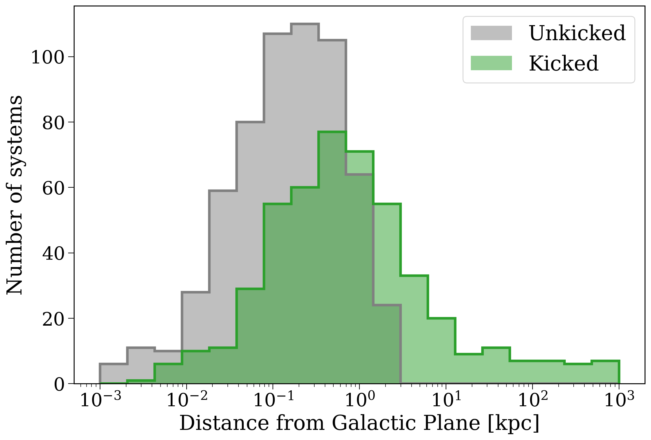
As one might expect, systems that received a supernova kick tend to get flung further away from the galactic plane!
Wrap-up#
And that’s all for this one, hope you enjoyed learning how to mask out your favourite population! Keep reading for the next tutorial on how to use these masks to re-run certain subpopulations in more detail.
Note
This tutorial was generated from a Jupyter notebook that can be found here.