Predicting observed Gaia population

Once you’ve computed the photometry of your sources it’s nice and simple to predict the portion of your population that observable by Gaia. Let’s talk about how to do it!

Learning Goals

By the end of this tutorial you should know how to:

• Apply the Gaia empirical selection function to your source photometry in a Population

Beware - extra dependencies required here!

You’ll need to have installed the extra dependencies of cogsworth to make predictions for Gaia. Check out the installation page for more details on how to do this! (You’ll probably just need to run pip install cogsworth[extras])

import cogsworth
import matplotlib.pyplot as plt
import numpy as np
import pandas as pd
import astropy.units as u

# this all just makes plots look nice
%config InlineBackend.figure_format = 'retina'

plt.rc('font', family='serif')
plt.rcParams['text.usetex'] = False
fs = 24

# update various fontsizes to match
params = {'figure.figsize': (12, 8),
          'legend.fontsize': fs,
          'axes.labelsize': fs,
          'xtick.labelsize': 0.9 * fs,
          'ytick.labelsize': 0.9 * fs,
          'axes.linewidth': 1.1,
          'xtick.major.size': 7,
          'xtick.minor.size': 4,
          'ytick.major.size': 7,
          'ytick.minor.size': 4}
plt.rcParams.update(params)
pd.options.display.max_columns = 999

Gaia observability

cogsworth uses the gaiaunlimited package to determine the Gaia observability of each source. The Gaia empirical selection gives the limiting magnitude for a given position on the sky and thus provides a more accurate estimate than a simple magnitude cut.

Once you’ve calculated the photometry (explained in the previous tutorial), working out which binaries are observable with Gaia is a simple function call away!

p = cogsworth.pop.Population(1000, use_default_BSE_settings=True)
p.create_population()
p.get_observables(filters=["Gaia_G_EDR3"], ignore_extinction=True,
                  assume_mw_galactocentric=True, silence_bounds_warning=True)

Run for 1000 binaries
Sampled 1335 binaries
[8e-03s] Sample initial binaries
[0.4s] Evolve binaries (run COSMIC)

Integrating orbits: 100%|██████████| 1341/1341 [00:01<00:00, 747.51it/s]

[2.6s] Integrate galactic orbits (run gala)
Overall: 3.0s

	Av_1	Av_2	M_abs_1	m_app_1	M_abs_2	m_app_2	Gaia_G_EDR3_app_1	Gaia_G_EDR3_app_2	teff_obs	log_g_obs	secondary_brighter	Gaia_G_EDR3_abs_1	Gaia_G_EDR3_abs_2
0	0.0	0.0	16.582948	34.693657	inf	inf	34.502030	inf	3.468207e+03	8.085400	False	16.391321	inf
1	0.0	0.0	8.492725	23.197668	8.595930	23.300873	23.223452	inf	3.697819e+03	4.832206	False	8.518510	inf
2	0.0	0.0	7.665989	22.561875	10.250501	25.146387	22.984300	inf	3.925716e+03	4.710860	False	8.088414	inf
3	0.0	0.0	inf	inf	inf	inf	inf	inf	1.833452e+06	-inf	False	inf	inf
4	0.0	0.0	10.191509	26.959628	10.728453	27.496572	27.004620	inf	3.630227e+03	5.071367	False	10.236500	inf
...	...	...	...	...	...	...	...	...	...	...	...	...	...
1330	0.0	0.0	9.165582	23.659866	9.471239	23.965523	23.740457	inf	3.614846e+03	4.924914	False	9.246173	inf
1331	0.0	0.0	4.753922	19.361943	10.944999	25.553021	19.240455	inf	5.758851e+03	4.431650	False	4.632433	inf
1332	0.0	0.0	8.515085	23.094082	8.815338	23.394335	23.112466	inf	3.707657e+03	4.836532	False	8.533468	inf
1333	0.0	0.0	9.588492	24.670505	11.342224	26.424237	25.232403	inf	3.555713e+03	4.969436	False	10.150390	inf
1334	0.0	0.0	15.181072	29.654803	9.152450	23.626181	24.162421	inf	3.687156e+03	4.939407	True	9.688690	inf

1335 rows × 13 columns

get_gaia_observed_bin_nums() return the bin_num s that correspond to the observable systems in two lists: one for bound binaries and disrupted primaries, and the other for disrupted secondaries.

Note that we need to specify the ra and dec for this function. In our case, let’s allow cogsworth to assume a Milky Way galactocentric frame for systems and automatically get their positions on the sky.

bound_prim_obs_nums, sec_obs_nums = p.get_gaia_observed_bin_nums(
    ra='auto', dec='auto'
)

Warning: the archive is unstable and we are working to resolve this issue. In case of questions, please contact the Gaia helpdesk: https://www.cosmos.esa.int/web/gaia/gaia-helpdesk

/Users/twagg/miniforge3/envs/cogsworth/lib/python3.11/site-packages/gaiaunlimited/selectionfunctions/apogee.py:7: UserWarning: pkg_resources is deprecated as an API. See https://setuptools.pypa.io/en/latest/pkg_resources.html. The pkg_resources package is slated for removal as early as 2025-11-30. Refrain from using this package or pin to Setuptools<81.
  import pkg_resources

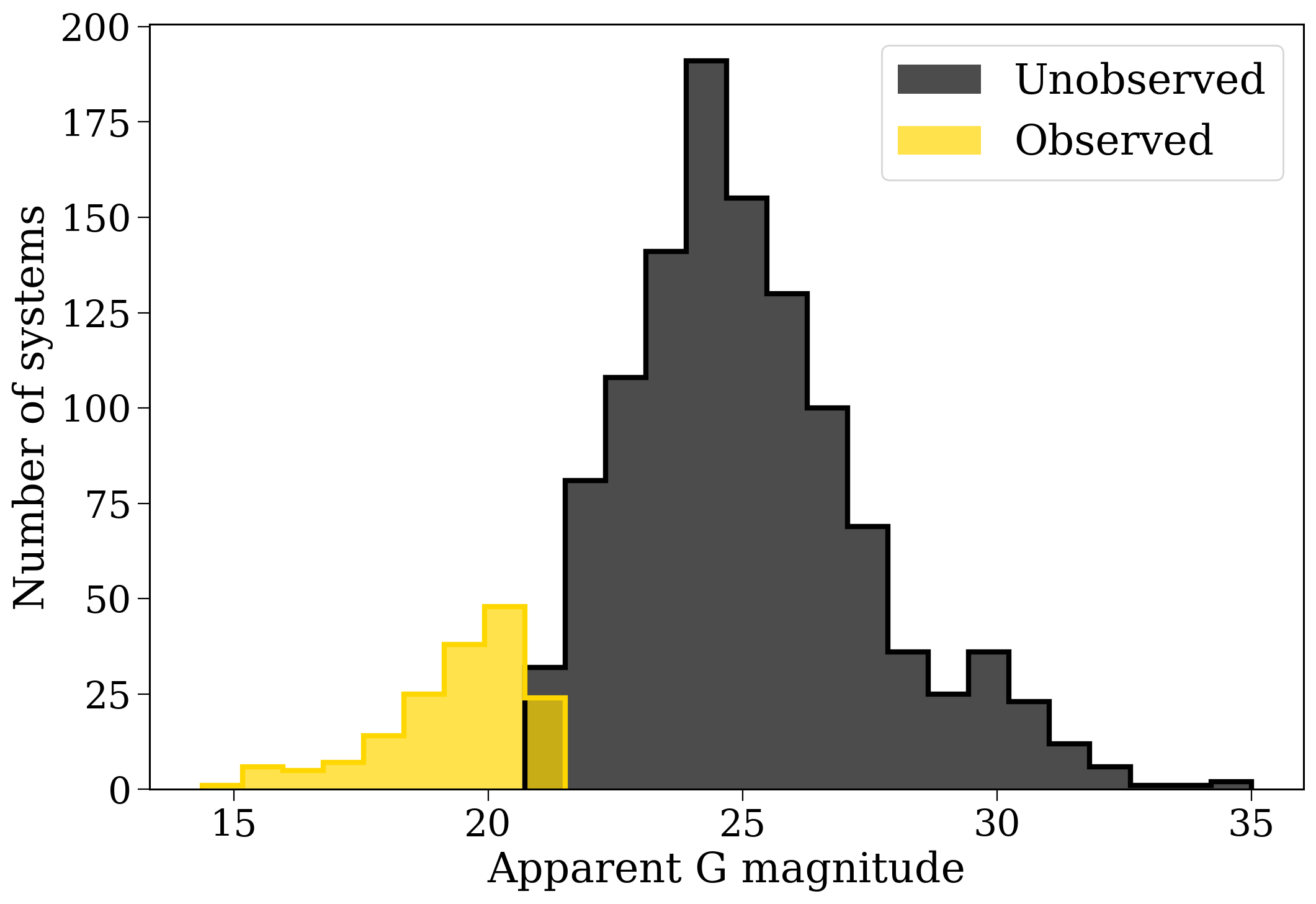
Let’s take a look at how the G magnitudes of the observed systems are different from those that aren’t observed.

obs_Gs = np.concatenate(
    (p.observables.loc[bound_prim_obs_nums]["Gaia_G_EDR3_app_1"].values,
     p.observables.loc[sec_obs_nums]["Gaia_G_EDR3_app_2"].values)
)
unobs_Gs = np.concatenate(
    (p.observables.loc[~p.observables.index.isin(bound_prim_obs_nums)]["Gaia_G_EDR3_app_1"].values,
     p.observables.loc[~p.observables.index.isin(sec_obs_nums)]["Gaia_G_EDR3_app_2"].values)
)

fig, ax = plt.subplots()

bins = np.linspace(12, 35, 30)
for G, colour, label in zip([unobs_Gs, obs_Gs],
                            ["black", "gold"],
                            ["Unobserved", "Observed"]):
    G = G[np.isfinite(G)]
    ax.hist(G, bins=bins[(bins > min(G) - 1) & (bins < max(G) + 1)],
            color=colour, alpha=0.7, label=label);
    ax.hist(G, bins=bins[(bins > min(G) - 1) & (bins < max(G) + 1)],
            color=colour, histtype="step", lw=3);
ax.legend()
ax.set(xlabel="Apparent G magnitude", ylabel="Number of systems")
plt.show()

f'Faintest observed magnitude: {obs_Gs.max():1.2f}'

'Faintest observed magnitude: 21.28'

f'Brightest unobserved magnitude: {unobs_Gs[~np.isnan(unobs_Gs)].min():1.2f}'

'Brightest unobserved magnitude: 20.94'

So, as one might guess, the observed systems are in general much brighter (lower magnitude). However, we can see that there are systems brighter than the faintest observed system that were NOT observed - this is exactly the idea we were discussing before where you position on the sky affects the magnitude limit.

Wrap-up

You should now know how to check the Gaia observability of your sources after that short little tutorial. Continue to the next tutorials to learn more about visualising your results with cogsworth!

Note

This tutorial was generated from a Jupyter notebook that can be found here.