Connecting `cogsworth` and `COMPAS`#

By default, cogsworth uses the COSMIC binary population synthesis code to perform binary stellar evolution. However, it is also possible to use the COMPAS code instead. This tutorial will guide you through the steps required to set up cogsworth to use COMPAS for binary population synthesis.

Learning Goals#

By the end of this tutorial you should know how to:

Run a simulation using COMPAS for binary population synthesis
Post-process a pre-run COMPAS simulation with cogsworth
Convert back and forth between Population and COMPASPopulation objects

[1]:

import cogsworth
import matplotlib.pyplot as plt
import numpy as np
import pandas as pd
import astropy.units as u

[2]:

# this all just makes plots look nice
%config InlineBackend.figure_format = 'retina'

plt.rc('font', family='serif')
plt.rcParams['text.usetex'] = False
fs = 24

# update various fontsizes to match
params = {'figure.figsize': (12, 8),
          'legend.fontsize': fs,
          'axes.labelsize': fs,
          'xtick.labelsize': 0.9 * fs,
          'ytick.labelsize': 0.9 * fs,
          'axes.linewidth': 1.1,
          'xtick.major.size': 7,
          'xtick.minor.size': 4,
          'ytick.major.size': 7,
          'ytick.minor.size': 4}
plt.rcParams.update(params)
pd.set_option('display.max_columns', None)

Set up your `COMPAS` installation#

First things first, we need to make sure you’ve installed COMPAS properly. Please make sure you’ve followed the instructions in the COMPAS documentation to install COMPAS on your system.

You can test that your installation is working by running the following command in your terminal:

$COMPAS_ROOT_DIR/COMPAS -v

If everything is set up correctly, you should see the version number of COMPAS printed to the terminal and some more information about that version.

Create a `COMPASPopulation` object#

Now that you have COMPAS installed, we can create a COMPASPopulation object in cogsworth. This object will allow us to run binary population synthesis using COMPAS. Let’s try this out with a simple example.

[3]:

p = cogsworth.COMPASPopulation(
    n_binaries=100,
    config_file=None,
    logfile_definitions=None,
    output_directory='./COMPAS_Output',
    final_kstar1=[13, 14],
)
p

[3]:

<COMPASPopulation - 100 systems - galactic_potential=MilkyWayPotential, SFH=Wagg2022>

Basic usage#

This COMPASPopulation object will work just how you might expect a Population object to work, but it will use COMPAS under the hood to perform the binary stellar evolution.

[4]:

p.create_population()

Run for 100 binaries
Ended up with 101 binaries with m1 > 0 solar masses
[1e-02s] Sample initial binaries
[5.6s] Evolve binaries (run COSMIC)

112it [00:00, 1213.51it/s]

[0.3s] Get orbits (run gala)
Overall: 5.9s

This command has:

Sampled initial binaries using COSMIC (with the default sampling_params in Population)
Sampled the star formation history of the galaxy
Performed binary stellar evolution using COMPAS
Performed galactic evolution using gala

It has also stored the output files from COMPAS in the specified output directory - so you can still use regular COMPAS tools to analyse the output if you wish.

[5]:

# print out the bpp table for the evolved binaries
p.bpp

[5]:

	tphys	mass_1	mass_2	kstar_1	kstar_2	sep	ecc	rad_1	rad_2	bin_num	evol_type	RRLO_1	RRLO_2	porb
1	0.000000	24.020449	21.735756	1	1	44840.919742	0.286859	6.492348	6.101377	1	1	0.000391	0.000351	162603.573692
1	7.444151	23.142886	21.197682	2	1	46272.529937	0.286859	17.246311	14.514294	1	2	0.001004	0.000811	173152.016069
1	7.455998	23.085489	21.196546	4	1	46333.694807	0.286859	489.402421	14.572830	1	2	0.028428	0.000814	173610.077052
1	8.245191	22.357717	21.132777	4	2	47176.983466	0.286859	1119.728293	15.883251	1	2	0.063453	0.000877	179987.108064
1	8.258944	22.339625	21.083359	4	4	47250.329325	0.286859	1122.834247	324.170660	1	2	0.063552	0.017869	180547.193520
...	...	...	...	...	...	...	...	...	...	...	...	...	...	...
101	33.888706	8.899451	4.390178	5	1	795.795399	0.000000	353.278256	2.376360	101	7	1.388577	0.006768	713.327595
101	33.888706	0.000000	0.000000	5	1	0.000000	0.000000	0.000000	0.000000	101	8	0.000000	0.000000	0.000000
101	33.888706	0.000000	0.000000	5	1	0.000000	0.000000	0.000000	0.000000	101	4	0.000000	0.000000	0.000000
101	33.888706	0.000000	0.000000	5	1	0.000000	0.000000	0.000000	0.000000	101	6	0.000000	0.000000	0.000000
101	33.888706	2.814327	4.390178	5	1	14.066892	0.000000	353.278256	2.376360	101	10	60.092987	0.495190	2.276871

1450 rows × 14 columns

[6]:

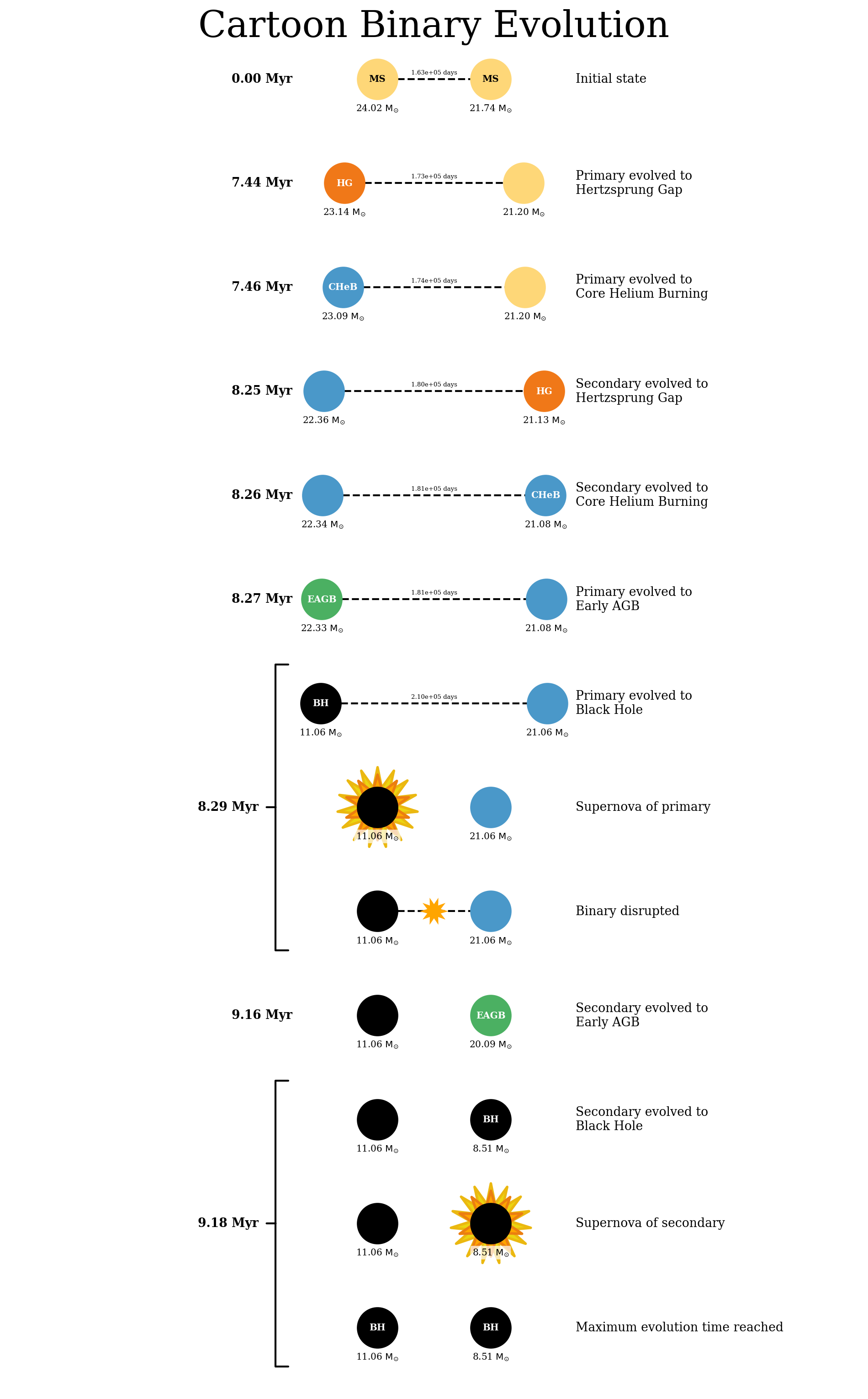
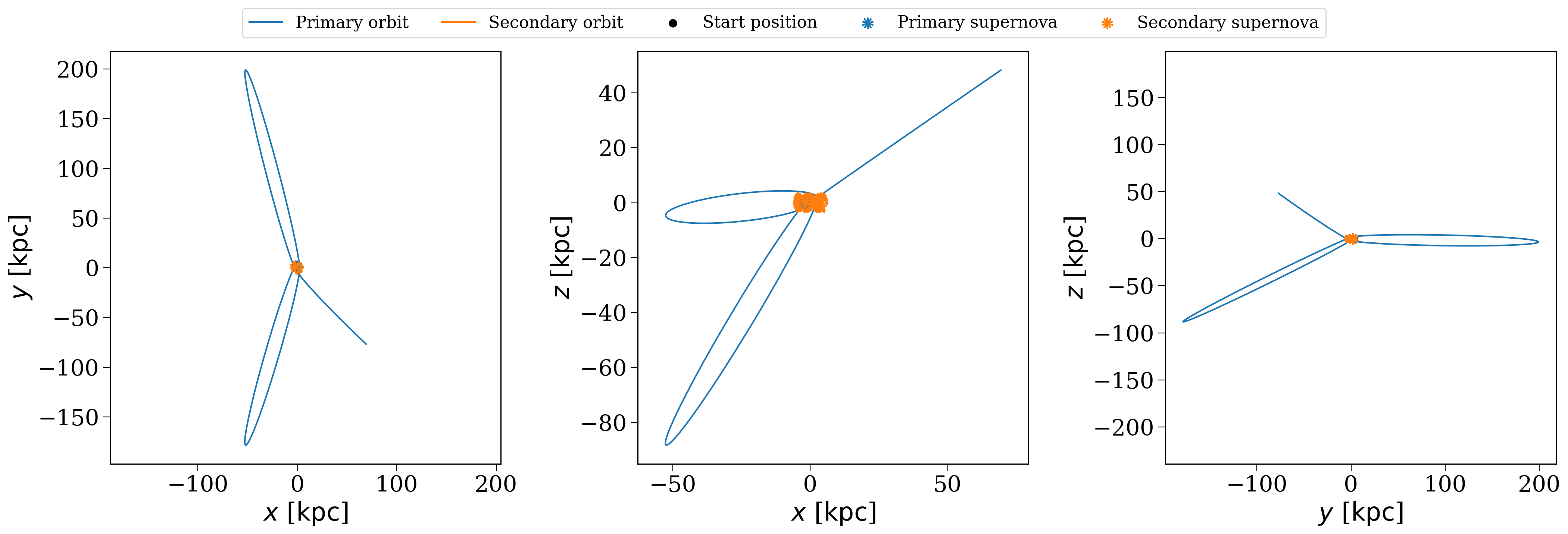
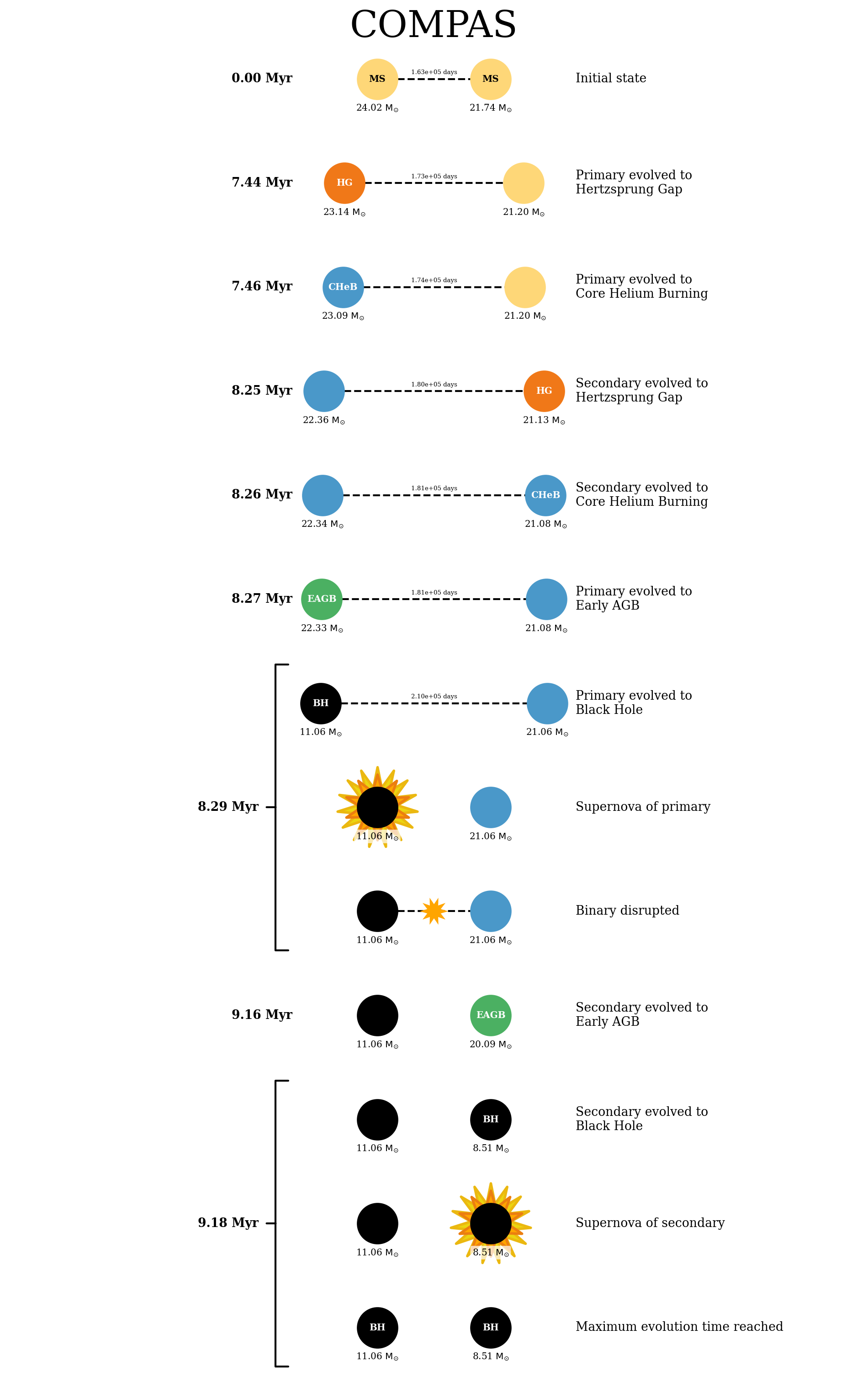
# plot the evolution and orbit of the first binary
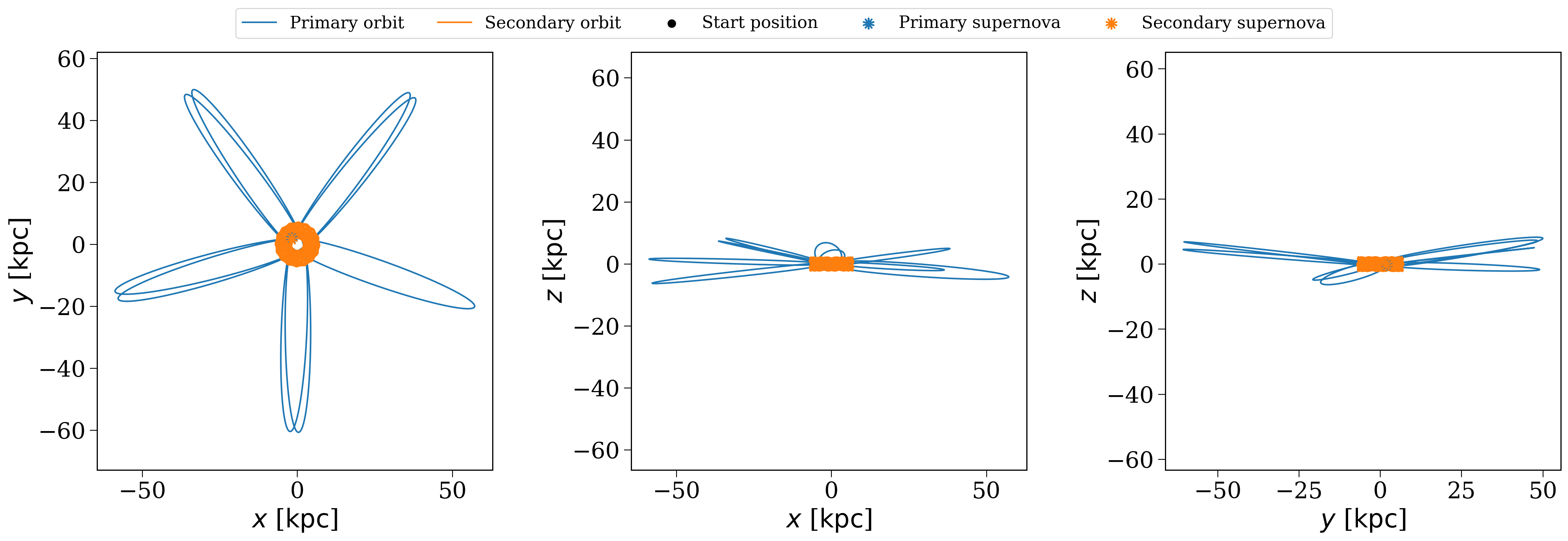
p.plot_cartoon_binary(p.bin_nums[0]);
p.plot_orbit(p.bin_nums[0]);

../../_images/tutorials_pop_synth_codes_compas_10_0.png

../../_images/tutorials_pop_synth_codes_compas_10_1.png

Change COMPAS settings#

You will have noticed above that the COMPASPopulation object takes a number of arguments that allow you to change the settings used by COMPAS. These are:

n_binaries: The number of binaries to simulate
config_file: The path to a COMPAS configuration file to use (by default it will use the one shipped with cogsworth)
logfile_definitions: The path to a COMPAS logfile definitions file to use (by default it will use the one shipped with cogsworth)
output_directory: The directory where the COMPAS output files will be saved

We can create our own config_file to change some of the settings used by COMPAS.

First, let’s download the default COMPAS config file from their GitHub repository.

[7]:

COMPAS_DEFAULT_CONFIG_URL = "https://raw.githubusercontent.com/TeamCOMPAS/COMPAS/refs/heads/dev/compas_python_utils/preprocessing/compasConfigDefault.yaml"
!wget {COMPAS_DEFAULT_CONFIG_URL} -O compas_config.yaml

--2026-02-02 18:06:25--  https://raw.githubusercontent.com/TeamCOMPAS/COMPAS/refs/heads/dev/compas_python_utils/preprocessing/compasConfigDefault.yaml
Resolving raw.githubusercontent.com (raw.githubusercontent.com)... 185.199.111.133, 185.199.108.133, 185.199.109.133, ...
Connecting to raw.githubusercontent.com (raw.githubusercontent.com)|185.199.111.133|:443... connected.
HTTP request sent, awaiting response... 200 OK
Length: 47542 (46K) [text/plain]
Saving to: ‘compas_config.yaml’

compas_config.yaml  100%[===================>]  46.43K  --.-KB/s    in 0.001s

2026-02-02 18:06:25 (39.8 MB/s) - ‘compas_config.yaml’ saved [47542/47542]

Now we can change some of those settings, let’s try turning stellar winds to a much older prescription by setting

compas_config.yaml#

--mass-loss-prescription: 'HURLEY'

Warning

Some settings are required for use with cogsworth!

In order to get an accurate bpp table from the COMPAS output, you must set --switch-log to True in your configuration file. You probably also want to use --evolve-unbound-systems as True to make sure you continue the stellar evolution after a disruption.

Now we can repeat our creation of the COMPASPopulation object with our new configuration file, but copy the initial binaries and initial galaxy from the previous run to make sure we are comparing identical initial populations.

[8]:

hurley_winds = cogsworth.COMPASPopulation(
    n_binaries=len(p),
    config_file='compas_config.yaml',
    logfile_definitions=None,
    output_directory='./COMPAS_Output_hurley_winds',
    final_kstar1=[13, 14],
)
hurley_winds._initial_binaries = p._initial_binaries.copy()
hurley_winds._initial_galaxy = p.initial_galaxy[:]
hurley_winds.perform_stellar_evolution()
hurley_winds.perform_galactic_evolution()

108it [00:00, 929.94it/s]

Now we can take the most massive initial binary star (where winds are important) and compare the binary evolution across the two runs for the same binary

[9]:

most_massive = p.bin_nums[p.initial_binaries["mass_1"].argmax()]

[10]:

p.bpp.loc[most_massive]

[10]:

	tphys	mass_1	mass_2	kstar_1	kstar_2	sep	ecc	rad_1	rad_2	bin_num	evol_type	RRLO_1	RRLO_2	porb
96	0.000000	58.532041	38.192146	1	1	18461.396587	0.030314	9.605389	7.443219	96	1	1.518579e-03	9.683532e-04	29544.224755
96	4.293896	50.578618	36.182795	2	1	20581.310343	0.030314	28.761856	13.774102	96	2	3.989142e-03	1.639439e-03	36718.889436
96	4.297866	19.567337	36.179806	7	1	32031.481222	0.030314	1.412270	13.790766	96	2	1.018207e-04	1.316009e-03	88940.084735
96	4.749850	16.282730	35.833516	8	1	34263.088751	0.030314	1.262747	16.483610	96	2	8.216884e-05	1.536435e-03	101764.550145
96	4.755994	16.143548	35.828816	14	1	34291.963093	0.030314	0.000068	16.532650	96	2	4.442848e-09	1.543025e-03	102034.161872
96	4.755994	16.143548	35.827699	14	1	34370.235012	0.032186	0.000068	16.532221	96	15	4.432757e-09	1.539459e-03	102384.802523
96	5.467048	16.143548	35.347952	14	2	34690.463062	0.032186	0.000068	20.036134	96	2	4.403607e-09	1.842185e-03	104301.532026
96	5.473791	16.143548	35.297624	14	4	34724.403175	0.032186	0.000068	812.811518	96	2	4.400549e-09	7.463236e-02	104505.722875
96	6.044947	16.143548	35.231830	14	5	34768.872783	0.032186	0.000068	964.511468	96	2	4.396552e-09	8.840625e-02	104773.563579
96	6.057153	16.143548	14.810516	14	14	57521.102596	0.032186	0.000068	0.000063	96	2	3.203301e-09	2.825320e-09	287227.012993
96	6.057153	16.143548	14.810516	14	14	57709.826479	0.032614	0.000068	0.000063	96	16	3.192825e-09	2.816080e-09	288641.738182
96	6.057153	16.143548	14.810516	14	14	57709.826479	0.032614	0.000068	0.000063	96	10	3.192825e-09	2.816080e-09	288641.738182

[11]:

hurley_winds.bpp.loc[most_massive]

[11]:

	tphys	mass_1	mass_2	kstar_1	kstar_2	sep	ecc	rad_1	rad_2	bin_num	evol_type	RRLO_1	RRLO_2	porb
96	0.000000	58.532041	38.192146	1	1	18461.396587	0.030314	9.605389	7.443219	96	1	1.518579e-03	9.683532e-04	29544.224755
96	4.755994	16.243548	35.827699	14	1	34300.213297	0.030314	0.000069	16.532221	96	15	4.474799e-09	1.540178e-03	101974.023468
96	6.057153	16.243548	14.873912	14	14	57398.903154	0.030437	0.000069	0.000063	96	16	3.231429e-09	2.842234e-09	285559.515438
96	6.057153	16.243548	14.873912	14	14	57398.903154	0.030437	0.000069	0.000063	96	10	3.231429e-09	2.842234e-09	285559.515438

As you can see, the evolution is very different with the different wind prescription!

Use a pre-run COMPAS simulation#

Often you may have already run a COMPAS simulation and want to use cogsworth to perform the galactic evolution and post-processing. This is easy to do with the COMPASPopulation object. You just need to provide the path to the COMPAS output directory with a specific method from the COMPASPopulation class. Here’s how to do that.

Let’s try:

Running a simulation without galactic evolution
Loading it back into a different object
Running the galactic evolution

[12]:

to_file = cogsworth.COMPASPopulation(
    n_binaries=100,
    final_kstar1=[13, 14],
    output_directory="./COMPAS_Output_IO",
)
to_file.sample_initial_binaries()
to_file.perform_stellar_evolution()

[13]:

from_file = cogsworth.COMPASPopulation.from_COMPAS_output("./COMPAS_Output_IO/COMPAS_Output.h5")
from_file

[13]:

<COMPASPopulation - 111 systems - galactic_potential=MilkyWayPotential, SFH=Wagg2022>

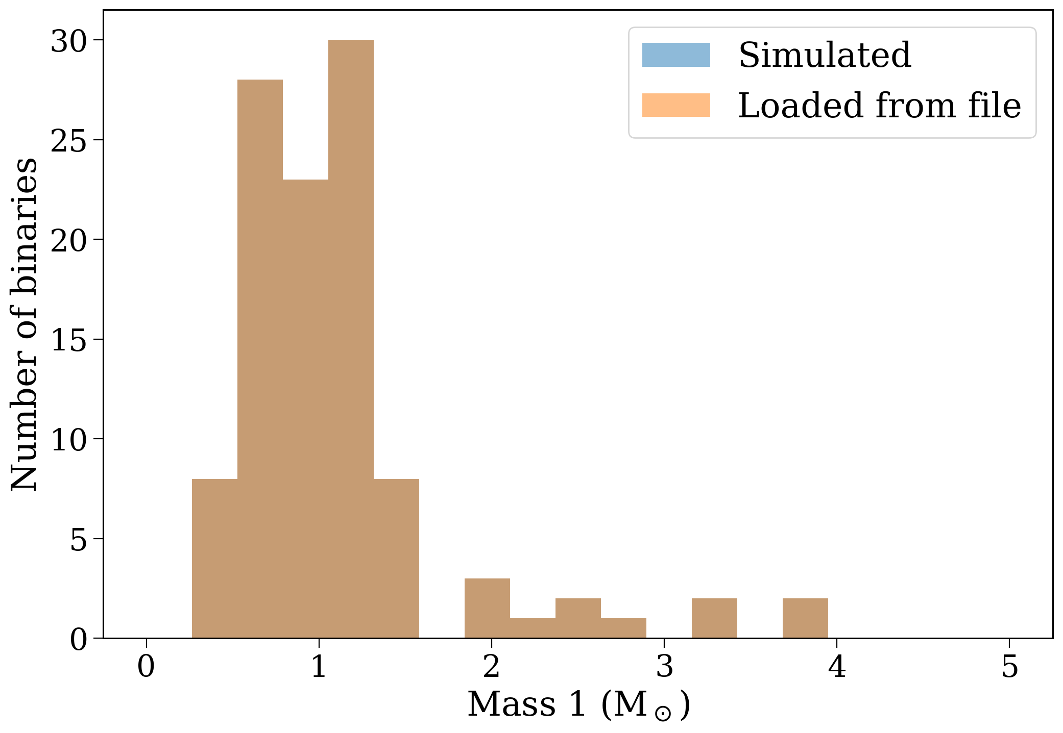
This loaded population can be demonstrated to be identical to the one that we ran it from:

[14]:

fig, ax = plt.subplots()

ax.hist(to_file.final_bpp["mass_1"], bins=np.linspace(0, 5, 20), alpha=0.5, label='Simulated')
ax.hist(from_file.final_bpp["mass_1"], bins=np.linspace(0, 5, 20), alpha=0.5, label='Loaded from file')

ax.set(
    xlabel='Mass 1 (M$_\odot$)',
    ylabel='Number of binaries',
)

ax.legend()
plt.show()

../../_images/tutorials_pop_synth_codes_compas_25_0.png

Plus now we can do the galactic evolution for this evolved population.

[16]:

from_file.perform_galactic_evolution()

122it [00:00, 1290.90it/s]

Convert between `COSMIC` and `COMPAS` populations#

You can easily convert between Population and COMPASPopulation objects using the provided methods. Here’s how to do that.

First, let’s convert our evolved COMPASPopulation object to a Population object.

[19]:

cosmic_p = p.to_Population()
cosmic_p

[19]:

<Population - 101 evolved systems - galactic_potential=MilkyWayPotential, sfh_model=Wagg2022>

Now let’s redo the stellar evolution and galactic orbit integration and see how things change!

[ ]:

cosmic_p.perform_stellar_evolution()
cosmic_p.perform_galactic_evolution()

109it [00:00, 1138.93it/s]

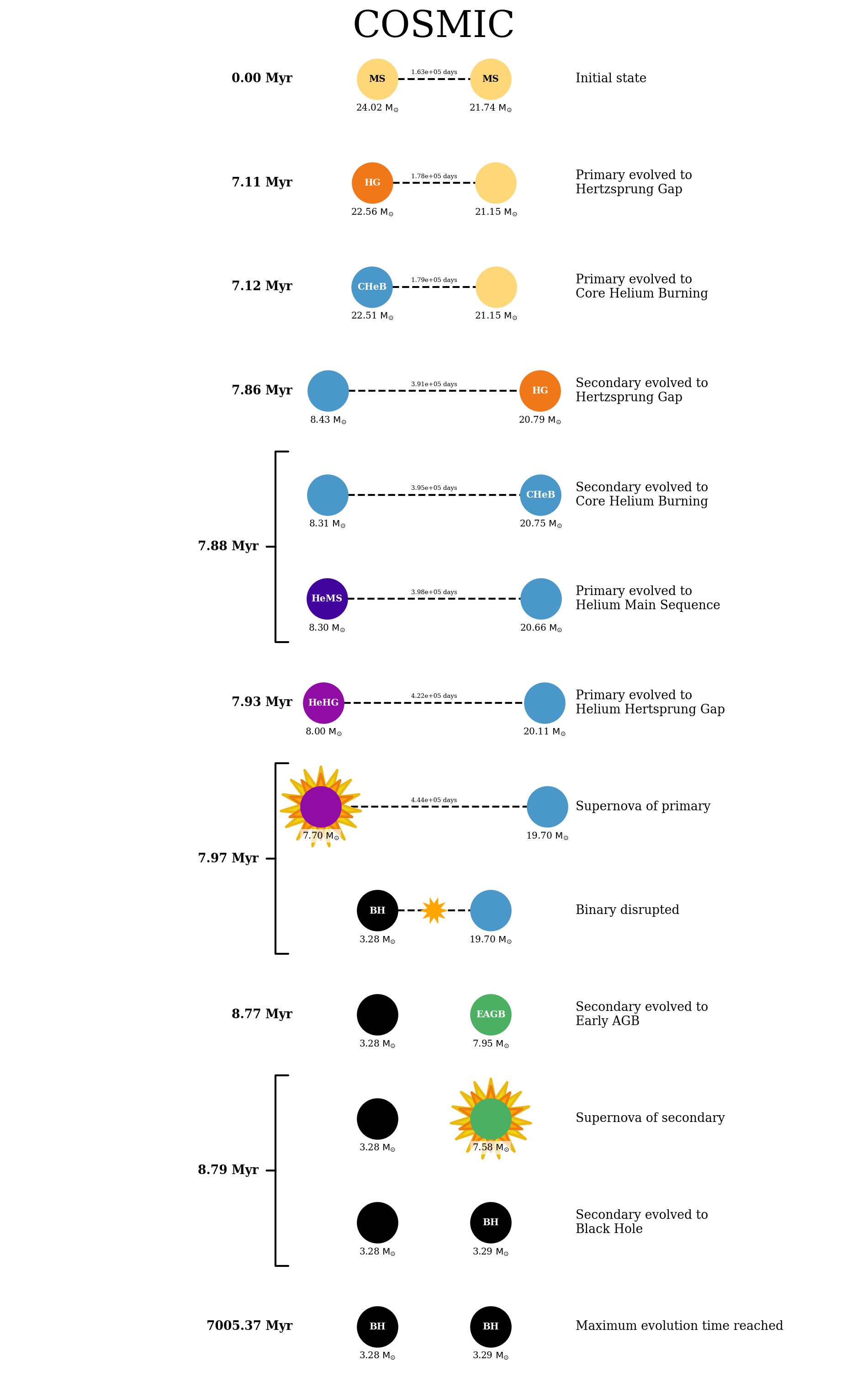
[23]:

cosmic_p.plot_cartoon_binary(cosmic_p.bin_nums[0], plot_title="COSMIC");
p.plot_cartoon_binary(cosmic_p.bin_nums[0], plot_title="COMPAS");

../../_images/tutorials_pop_synth_codes_compas_32_0.png

../../_images/tutorials_pop_synth_codes_compas_32_1.png

[25]:

cosmic_p.plot_orbit(cosmic_p.bin_nums[0]);
p.plot_orbit(cosmic_p.bin_nums[0]);

../../_images/tutorials_pop_synth_codes_compas_33_0.png

../../_images/tutorials_pop_synth_codes_compas_33_1.png

As is probably evident (these are randomly generated each time I build the docs, so not for sure), COMPAS and COSMIC give different results for the same inputs!

You can also do the opposite and convert a COSMIC population back to a COMPAS one.

[24]:

compas_from_cosmic = cosmic_p.to_COMPASPopulation()
compas_from_cosmic

[24]:

<COMPASPopulation - 101 evolved systems - galactic_potential=MilkyWayPotential, sfh_model=Wagg2022>

Wrap-up#

And that’s a wrap! You’ve now learned how to use cogsworth with COMPAS for binary population synthesis. You should now be able to set up your own COMPASPopulation objects, run simulations, and convert between Population and COMPASPopulation objects. Happy simulating!

Note

This tutorial was generated from a Jupyter notebook that can be found here.

Connecting cogsworth and COMPAS#

Learning Goals#

Set up your COMPAS installation#

Create a COMPASPopulation object#