Identifying `LISA` sources in your population#

In this tutorial we’ll discuss how to turn your Population into a collection of LISA sources and see which ones could be detectable from their gravitational wave emission during inspiral.

Learning Goals#

By the end of this tutorial you should know how to:

Convert your Population to a LEGWORK Source class
Calculate the LISA signal-to-noise ratio for each of your sources

Beware - extra dependencies required here!

You’ll need to have installed the extra dependencies of cogsworth to calculate LISA SNRs. Check out the installation page for more details on how to do this! (You’ll probably just need to run pip install cogsworth[extras])

[1]:

import cogsworth
import matplotlib.pyplot as plt
import numpy as np
import pandas as pd
import astropy.units as u

[24]:

# this all just makes plots look nice
%config InlineBackend.figure_format = 'retina'

plt.rc('font', family='serif')
plt.rcParams['text.usetex'] = False
fs = 24

# update various fontsizes to match
params = {'figure.figsize': (12, 8),
          'legend.fontsize': fs,
          'axes.labelsize': fs,
          'xtick.labelsize': 0.9 * fs,
          'ytick.labelsize': 0.9 * fs,
          'axes.linewidth': 1.1,
          'xtick.major.size': 7,
          'xtick.minor.size': 4,
          'ytick.major.size': 7,
          'ytick.minor.size': 4}
plt.rcParams.update(params)
pd.options.display.max_columns = 999

Converting to LISA sources#

Since I also wrote a Python package for calculating signal-to-noise ratios of stellar-mass binaries in LISA (our good friend LEGWORK) I thought it could be nice to smoothly link the two of them. This means it actually just requires a single class method call to turn your population into sources for LEGWORK!

[15]:

p = cogsworth.pop.Population(1000, final_kstar1=[10, 11, 12],
                             use_default_BSE_settings=True)
p.create_population()

Run for 1000 binaries
Ended up with 1084 binaries with m1 > 0 solar masses
[4e-02s] Sample initial binaries
[1.8s] Evolve binaries (run COSMIC)

1098it [00:05, 205.98it/s]

[7.1s] Get orbits (run gala)
Overall: 9.0s

[34]:

# return a collection of LEGWORK sources for all bound binaries in the population
sources = p.to_legwork_sources(assume_mw_galactocentric=True)
sources

[34]:

<legwork.source.Source at 0x756839c58820>

And that’s it! Now we can use LEGWORK to learn more about these sources.

Using `LEGWORK` to calculate SNRs#

Let’s explore a little bit of what you might want to do with LEGWORK here. But first I’m going to cheat and put every binary at 1pc just so that we have a nonzero population with SNR > 1 even though I evolved very few binaries.

[35]:

# return a collection of LEGWORK sources for all bound binaries in the population
sources = p.to_legwork_sources(distances=1 * u.pc * np.ones(len(p)))
sources

[35]:

<legwork.source.Source at 0x756842394b50>

Now we calculate the SNR with the following and let’s print out the top three sources

[41]:

sources.get_snr()
np.sort(sources.snr)[-3:]

[41]:

array([209.76833486, 295.16467453, 463.0752157 ])

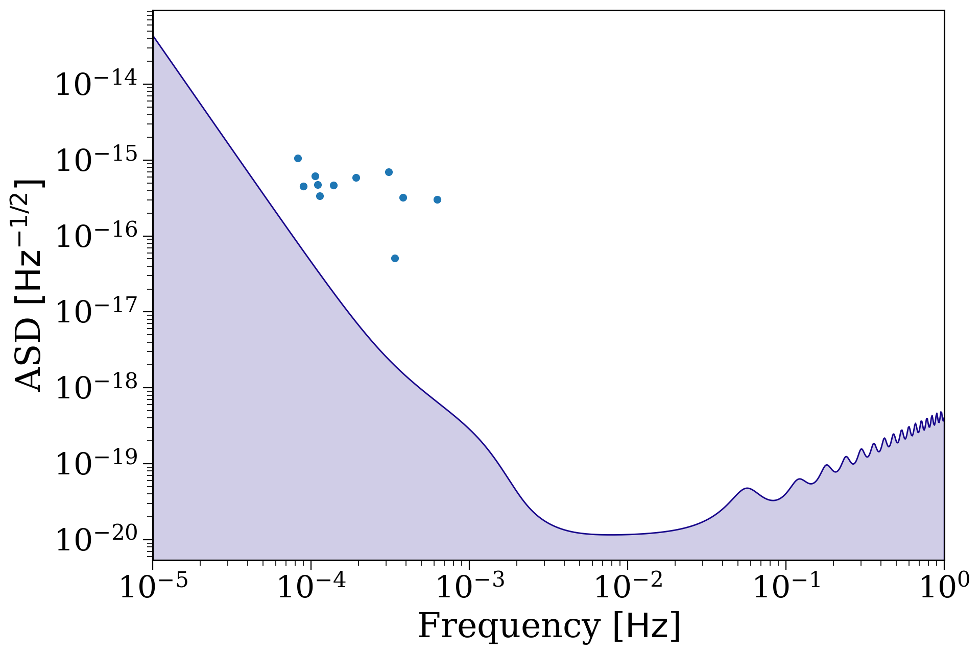
You can also plot these sources on the sensitivity curve. Let’s plot up the ones that meet a threshold of SNR = 7.

[48]:

sources.plot_sources_on_sc(snr_cutoff=7);

../../_images/tutorials_misc_lisa_12_0.png

Wrap-up#

And that’s all for interfacing cogsworth with LEGWORK - check out the LEGWORK documentation to learn more about how you can predict LISA signals from your binaries.

Note

This tutorial was generated from a Jupyter notebook that can be found here.

Identifying LISA sources in your population#