Using distribution function based star formation histories

In this tutorial we’ll discuss how to create a distribution function based star formation history (SFH) using the cogsworth.sfh module. These SFHs are based on analytic distribution functions (DFs) for stellar systems in equilibrium, and allow you to create more realistic SFHs that take into account the dynamics of the system.

Learning Goals

By the end of this tutorial you should know how to:

• Create a distribution function based SFH using classes that inherit from the cogsworth.sfh.DistributionFunctionBasedSFH class

• Use pre-defined SFHs for specific systems, such as the Milky Way disc and dwarf spheroidal galaxies

• Apply these SFHs to generate stellar populations with realistic spatial and kinematic distributions with a cogsworth.sfh.Population

Beware - extra dependencies required here!

You’ll need to have installed the extra dependencies of cogsworth to use distribution function based star formation histories. Check out the installation page for more details on how to do this! (You’ll probably just need to run pip install cogsworth[extras])

import cogsworth
import matplotlib.pyplot as plt
import numpy as np
import pandas as pd
import astropy.units as u
import gala.potential as gp
from gala.units import galactic

import agama
agama.setUnits(**{k: galactic[k] for k in ['length', 'mass', 'velocity']})

# this all just makes plots look nice
%config InlineBackend.figure_format = 'retina'

plt.rc('font', family='serif')
plt.rcParams['text.usetex'] = False
fs = 24

# update various fontsizes to match
params = {'figure.figsize': (12, 8),
          'legend.fontsize': fs,
          'axes.labelsize': fs,
          'xtick.labelsize': 0.9 * fs,
          'ytick.labelsize': 0.9 * fs,
          'axes.linewidth': 1.1,
          'xtick.major.size': 7,
          'xtick.minor.size': 4,
          'ytick.major.size': 7,
          'ytick.minor.size': 4}
plt.rcParams.update(params)
pd.options.display.max_columns = 999

Why use distribution function based SFHs?

The simpler star formation histories in cogsworth (e.g., Wagg2022 and ConstantUniformDisc) are useful for generating populations quickly, especially those that are short lived. For longer lived populations, however, it is often desirable to have a more realistic spatial and kinematic distribution for your stars. This is especially true if you want to model populations in specific systems, such as the Milky Way disc or dwarf spheroidal galaxies. We’ll illustrate this in more detail below.

The basic limitation with the simpler SFHs is that they do not take into account the dynamics of the system. In Wagg2022, for example, stars are born with velocities that are a combination of the circular velocity at their birth radius and a random velocity dispersion drawn from a Gaussian. This may not be entirely consistent with the velocity a star should have that a given location.

What is a distribution function?

Simply put, a distribution function describes the density of stars in phase space. In other words, it tells you how many stars you can expect to find in a given volume of position and velocity space. For a system in equilibrium, the distribution function is time independent, and can be used to generate a population of stars that are consistent with the gravitational potential of the system.

Distribution function based SFHs in cogsworth use functions of actions and pass them to agama for sampling.

Using distribution function based SFHs

Simple dwarf galaxy

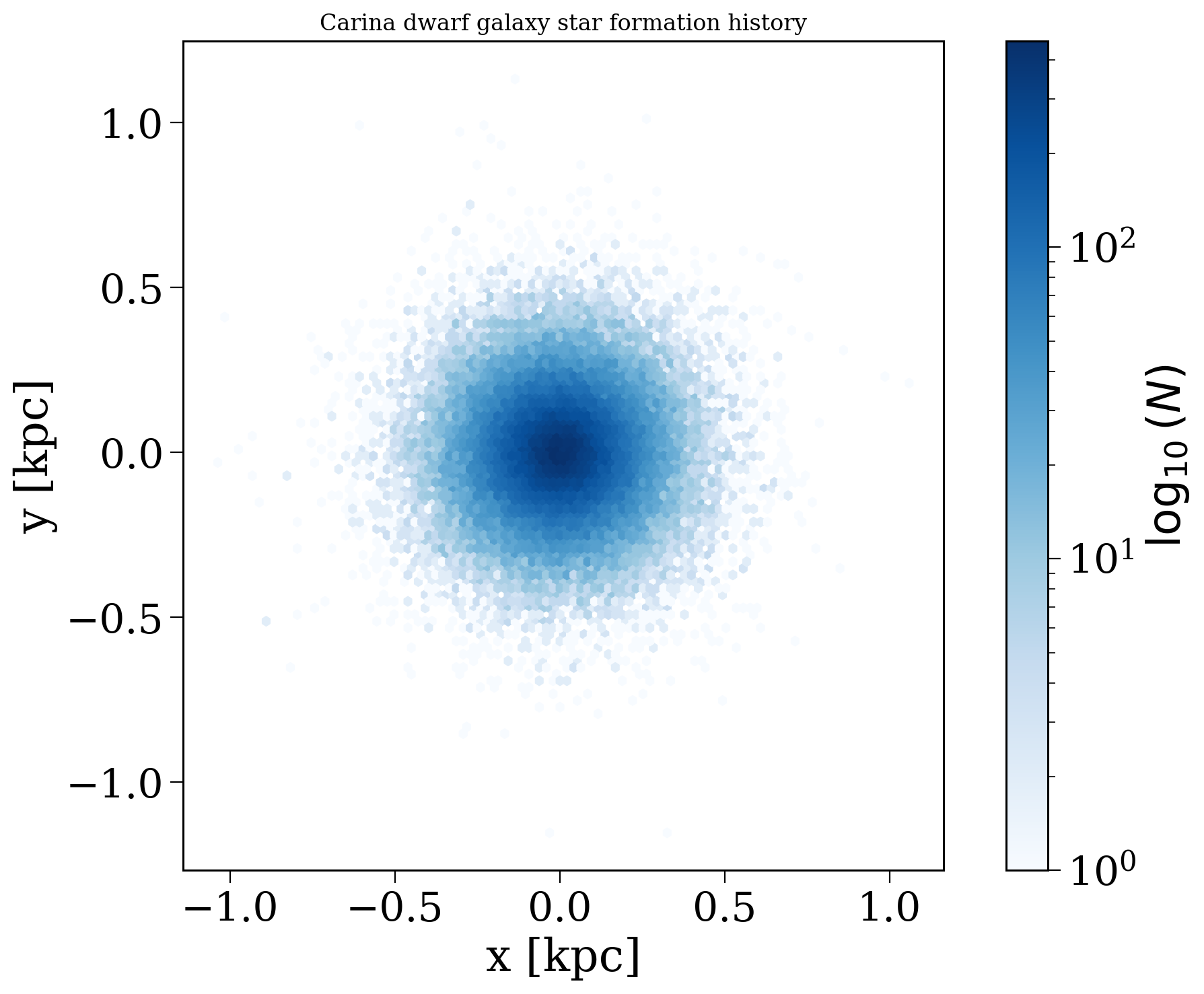
Let’s start by creating a simple SFH based on the Carina Dwarf galaxy, which is built into cogsworth as the CarinaDwarf class.

carina = cogsworth.sfh.CarinaDwarf(fixed_Z=0.001, tau_min=6.9 * u.Gyr, galaxy_age=7 * u.Gyr)
carina.sample(100_000)

fig, ax = plt.subplots()

hex = ax.hexbin(carina.x, carina.y, gridsize=100, cmap='Blues', mincnt=1, bins='log')
cb = fig.colorbar(hex, ax=ax, label=r'$\log_{10}(N)$')
ax.set_xlabel('x [kpc]')
ax.set_ylabel('y [kpc]')
ax.set_title('Carina dwarf galaxy star formation history')
ax.set_aspect('equal')
plt.show()

More complex SFHs

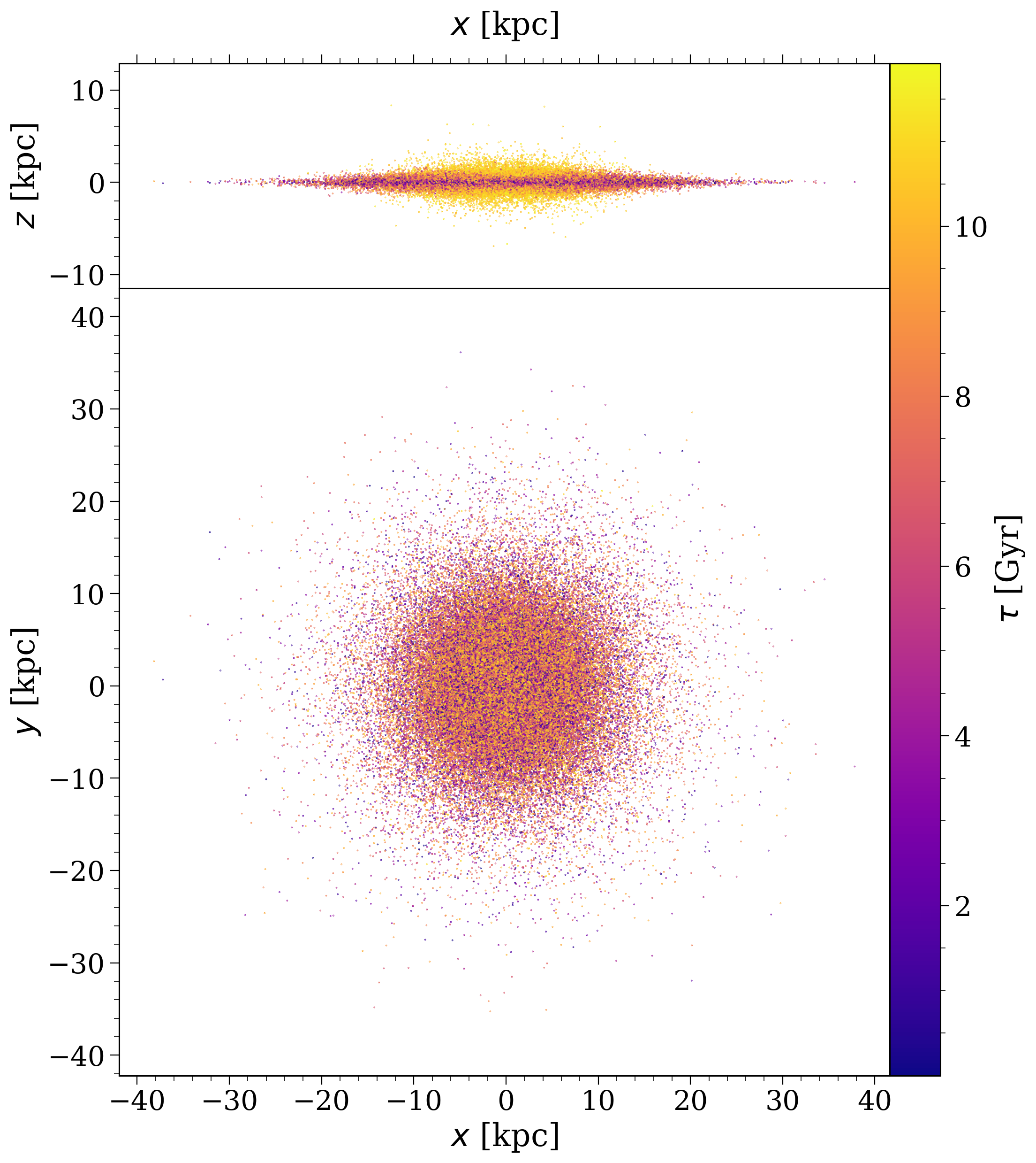
There are also more complex SFHs that model, for example, the Milky Way discs. We can try this out with the SandersBinney2015 class, which is based on the SFH from Sanders & Binney (2015). This class creates both discs and also accounts for some time dependence. As you may expect, this makes it slightly slower to sample from.

The distribution function for Sanders & Binney (2015) can be written as

\[f(\mathbf{J}) = \frac{1}{8 \pi^3} [1 + \tanh(J_\phi / L_0)] \cdot \frac{\Omega}{R_d^2 \kappa^2} e^{-R_c / R_d} \cdot \frac{\kappa}{\sigma_r^2} e^{-\kappa J_r / \sigma_r^2} \cdot \frac{\nu}{\sigma_z^2} e^{-\nu J_r / \sigma_z^2}\]

You can read the paper for details on the exact parameters, but suffice to say they take on different values for the thin and thick disc and also evolve with time.

sb15 = cogsworth.sfh.SandersBinney2015(potential=gp.MilkyWayPotential(version='v2'), verbose=True)
sb15.sample(100_000)

Pre-computing lookback time, guiding radius and frequency interpolations
Initiating sampling procedure
  Sampling 80984 stars from the thin_disc
    Sampling 9703 stars with lookback times between 0.00 Gyr and 2.00 Gyr
    Sampling 12396 stars with lookback times between 2.00 Gyr and 4.00 Gyr
    Sampling 15485 stars with lookback times between 4.00 Gyr and 6.00 Gyr
    Sampling 19498 stars with lookback times between 6.00 Gyr and 8.00 Gyr
    Sampling 23902 stars with lookback times between 8.00 Gyr and 10.00 Gyr
  Sampling 19016 stars from the thick_disc
    Sampling 19016 stars with lookback times between 10.00 Gyr and 12.00 Gyr

sb15.plot(colour_by=sb15.tau.value, cbar_norm=None, cbar_label=r'$\tau$ [Gyr]')

(<Figure size 1247.5x1400 with 3 Axes>,
 array([<Axes: xlabel='$x$ [kpc]', ylabel='$z$ [kpc]'>,
        <Axes: xlabel='$x$ [kpc]', ylabel='$y$ [kpc]'>], dtype=object))

Custom distribution functions

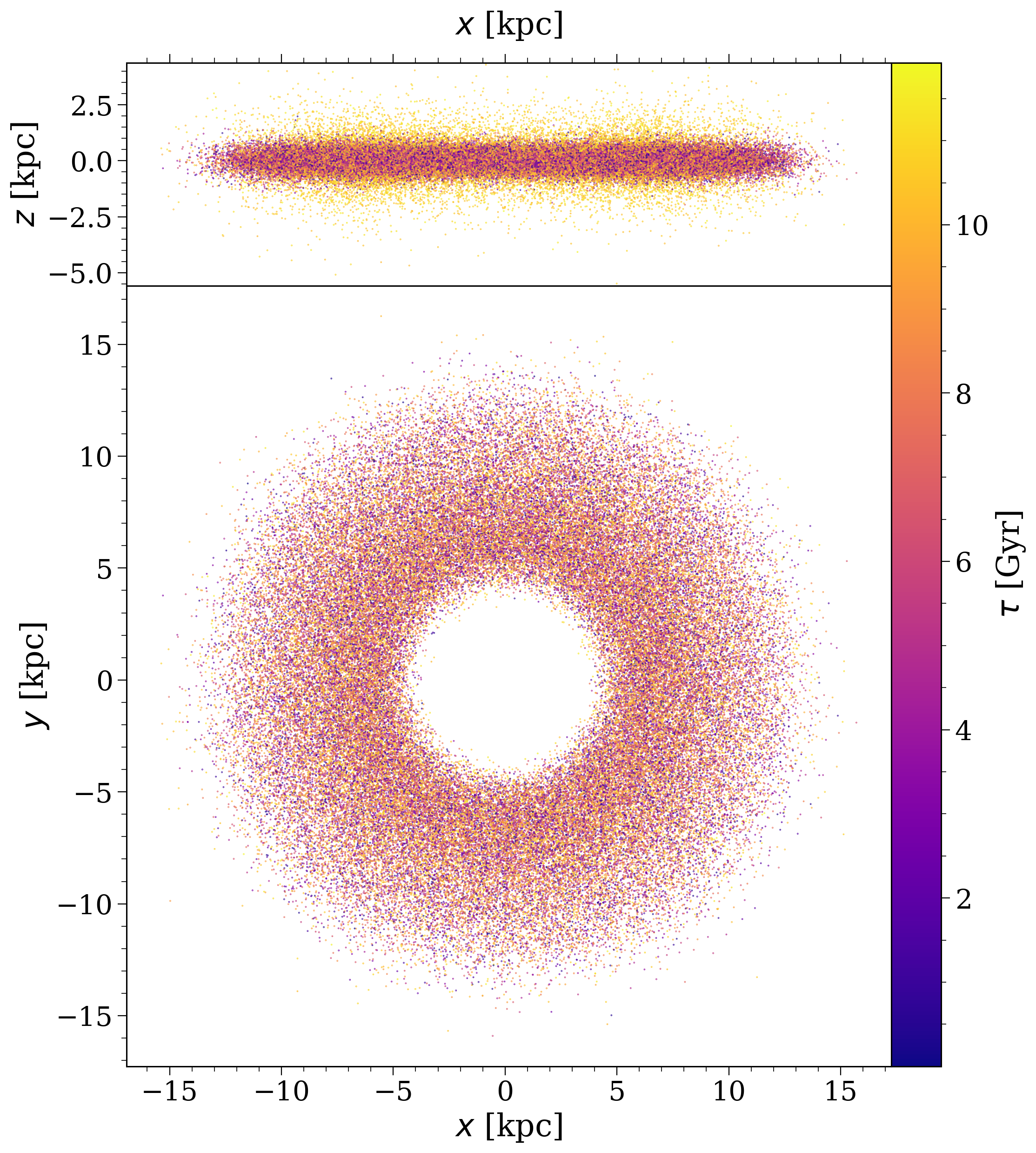
You can also create your own distribution function based SFH as long as you have a definition for the distribution function of the form f(J) where J are the actions. Let’s try this out.

Below we create a new class called MWAnnulus that inherits from SandersBinney2015 but modifies the distribution function to only create stars in an annulus around the solar radius. This is done by overriding the _generate_df method to include a cut on the azimuthal action, J_phi.

class MWAnnulus(cogsworth.sfh.SandersBinney2015):
    def _generate_df(self, J, component, tau):
        """Generate a distribution function for a given component and lookback time

        Follows `Sanders & Binney 2015 <https://ui.adsabs.harvard.edu/abs/2015MNRAS.449.3479S/abstract>`_
        Eq. 3.1.

        Parameters
        ----------
        J : `array-like`, shape (N, 3)
            Actions in (J_r, J_phi, J_z) in units of kpc^2 / Myr
        component : `str`
            Either "thin_disc" or "thick_disc"
        tau : :class:`~astropy.units.Quantity` [time]
            Lookback time

        Returns
        -------
        df_val : `array-like`, shape (N,)
            Value of the distribution function at the given actions
        """
        assert component in ["thin_disc", "thick_disc"], "Component must be 'thin_disc' or 'thick_disc'"

        J_r, J_z, J_phi = J.T

        # only compute the DF where the prior interpolations are valid
        df_val = np.full_like(J_r, np.nan)
        valid = (J_phi >= 1e-5) & (J_phi <= 100)

        R_d = 3.45 if component == "thin_disc" else 2.31
        L_0 = 0.01

        # get guiding radii
        R_g = np.zeros_like(J_r)
        R_g[valid] = self._guiding_radius_interp(J_phi[valid])
        valid &= (R_g >= 1e-2) & (R_g <= 100)
        R_g = R_g[valid]

        # get frequencies at guiding radii based on potential
        omega = self._omega_interp(R_g)
        kappa = self._kappa_interp(R_g)
        nu = self._nu_interp(R_g)

        # time dependent velocity dispersions
        kms_to_kpcMyr = (u.km / u.s).to(u.kpc / u.Myr)
        sigma_R = self._get_sigma_i("R", R_g, tau, component) * kms_to_kpcMyr
        sigma_z = self._get_sigma_i("z", R_g, tau, component) * kms_to_kpcMyr

        # construct DF
        prefactor = 1 / (8 * np.pi**3) * (1 + np.tanh(J_phi[valid] / L_0))          # no units
        exp_terms = [
            omega / (R_d**2 * kappa**2) * np.exp(-R_g / R_d),                       # units of Myr/kpc^2
            (kappa / sigma_R**2) * np.exp(-kappa * J_r[valid] / sigma_R**2),        # units of Myr/kpc^2
            (nu / sigma_z**2) * np.exp(-nu * J_z[valid] / sigma_z**2)               # units of Myr/kpc^2
        ]
        df_val[valid] = prefactor * np.prod(exp_terms, axis=0)                      # units of Myr^3/kpc^6


        ##########################
        ####
        ## LOOK HERE!
        ###
        ## This is where we modify the DF to only include stars in an annulus
        ## around the solar radius. We do this by cutting on J_phi.

        df_val[(J_phi < 1.17) | (J_phi > 2.8)] = 0.0

        ##########################

        return df_val

ring = MWAnnulus(potential=gp.MilkyWayPotential(version='v2'), verbose=True, time_bins=1)
ring.sample(100_000)

Pre-computing lookback time, guiding radius and frequency interpolations
Initiating sampling procedure
  Sampling 81029 stars from the thin_disc
    Sampling 81029 stars with lookback times between 0.00 Gyr and 10.00 Gyr
  Sampling 18971 stars from the thick_disc
    Sampling 18971 stars with lookback times between 10.00 Gyr and 12.00 Gyr

ring.plot(colour_by=ring.tau.value, cbar_norm=None, cbar_label=r'$\tau$ [Gyr]')

(<Figure size 1247.5x1400 with 3 Axes>,
 array([<Axes: xlabel='$x$ [kpc]', ylabel='$z$ [kpc]'>,
        <Axes: xlabel='$x$ [kpc]', ylabel='$y$ [kpc]'>], dtype=object))

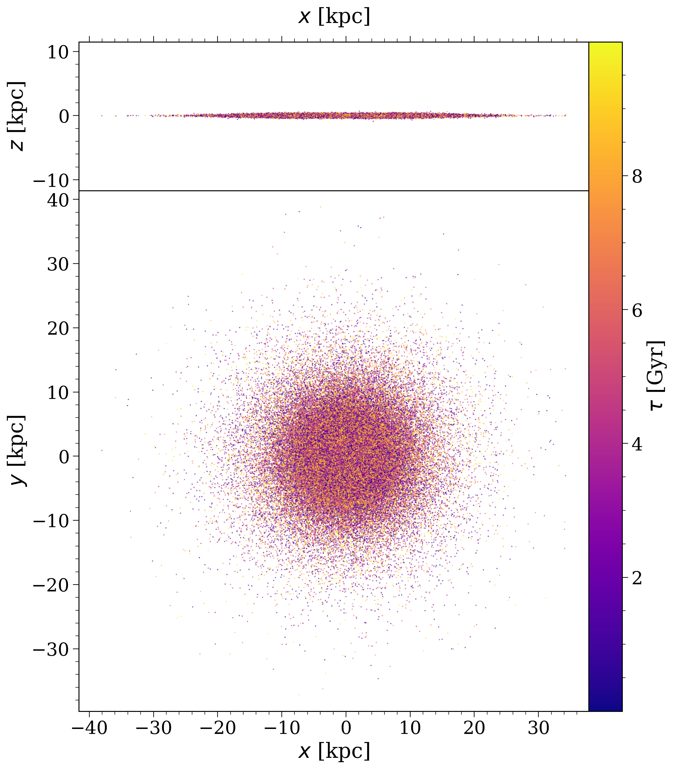
Alternatively, we can some of the builtin DFs in agama by passing a dictionary

class SimpleQID(cogsworth.sfh.DistributionFunctionBasedSFH):
    def draw_lookback_times(self, size, component=None):
        self._tau = np.random.uniform(0, 10, size) * u.Gyr
        return self._tau

    def get_metallicity(self):
        self._Z = np.repeat(0.02, len(self._tau))
        return self._Z

qid = SimpleQID(
    potential=gp.MilkyWayPotential(version='v2'),
    df={
        'type': 'QuasiIsothermal',
        'Rdisk': 3.45,
        'Rsigmar': 7.8,
        'Rsigmaz': 7.8,
        'sigmar0': (48.3*u.km/u.s).decompose(galactic).value,
        'sigmaz0': (30.7*u.km/u.s).decompose(galactic).value,
        'Sigma0': 1.0,
    }
)
qid.sample(100_000)

qid.plot(colour_by=qid.tau.value, cbar_norm=None, cbar_label=r'$\tau$ [Gyr]')

(<Figure size 1247.5x1400 with 3 Axes>,
 array([<Axes: xlabel='$x$ [kpc]', ylabel='$z$ [kpc]'>,
        <Axes: xlabel='$x$ [kpc]', ylabel='$y$ [kpc]'>], dtype=object))

Using distribution function based SFHs with populations

Now, allow me to prove to you that this was worth it! Let’s create a population using the Sanders & Binney (2015) SFH and compare it to one created with the simpler Wagg2022 SFH.

Fair warning, both of these next cells may take a few minutes to run. Though, you’ll note that the overall runtime is still dominated by the binary evolution, not the SFH.

p_sb15 = cogsworth.pop.Population(
    10_000,
    sfh_model=cogsworth.sfh.SandersBinney2015(
        potential=gp.MilkyWayPotential(version='v2'),
        time_bins=5
    ),
    use_default_BSE_settings=True
)
p_sb15.create_population()

Run for 10000 binaries
Sampled 13184 binaries
[2e+00s] Sample initial binaries
[2.6s] Evolve binaries (run COSMIC)

Integrating orbits: 100%|██████████| 13229/13229 [00:26<00:00, 494.19it/s]
cogsworth warning: 1 orbit(s) failed numerical integration, removing them. This can occur due to NaNs in stellar evolution or extreme orbits (e.g. passing directly through the galactic centre) that Gala cannot handle. Information for these systems was saved to `./failed_integration_binaries.h5`. This includes their initial_binaries, bpp, kick_info, and initial galaxy objects.

[34.6s] Integrate galactic orbits (run gala)
Overall: 39.1s

p_wagg = cogsworth.pop.Population(10_000, sfh_model=cogsworth.sfh.Wagg2022(), use_default_BSE_settings=True)
p_wagg.create_population()

Run for 10000 binaries
Sampled 13228 binaries
[4e-02s] Sample initial binaries
[2.6s] Evolve binaries (run COSMIC)

Integrating orbits: 100%|██████████| 13280/13280 [00:33<00:00, 396.12it/s]
cogsworth warning: 2 orbit(s) failed numerical integration, removing them. This can occur due to NaNs in stellar evolution or extreme orbits (e.g. passing directly through the galactic centre) that Gala cannot handle. Information for these systems was saved to `./failed_integration_binaries_1.h5`. This includes their initial_binaries, bpp, kick_info, and initial galaxy objects.

[44.3s] Integrate galactic orbits (run gala)
Overall: 47.0s

With both of those populations complete, let’s compare their spatial distributions at birth and at present day. We’ll remove anything that received a kick during its evolution to make the comparison cleaner. Ideally we should see that the initial and final distributions are similar, as both SFHs should be in equilibrium with the Milky Way potential.

fig, axes = plt.subplots(2, 1, figsize=(12, 12))

# loop over both populations
for pop, pop_name, ax in zip([p_wagg, p_sb15], ["Wagg+2022", "Sanders & Binney 2015"], axes):

    # remove anything that got a kick
    were_kicked = pop.bpp[pop.bpp["evol_type"].isin([15, 16])]["bin_num"].unique()
    unkicked = ~np.isin(pop.bin_nums, were_kicked)

    # plot initial and final z distributions
    for z, c, l in zip([pop.initial_galaxy.z[unkicked].value,
                        pop.final_pos[:, 2][:len(pop)][unkicked].value],       # [:len(pop)] removes disrupted secondaries
                       ["tab:blue", "tab:purple"],
                       ["Initial", "Final"]):
        ax.hist(z, bins=np.linspace(-2.5, 2.5, 100), histtype="step", color=c, label=l, lw=2)
        ax.hist(z, bins=np.linspace(-2.5, 2.5, 100), color=c, alpha=0.2)

    ax.legend()
    ax.set_xlabel(r"$z$ [kpc]")
    ax.set_ylabel("Counts")
    ax.set_ylim(0, 2000)

    ax.annotate(pop_name, xy=(0.03, 0.95), xycoords='axes fraction', va='top', ha='left', fontsize=20)

plt.show()

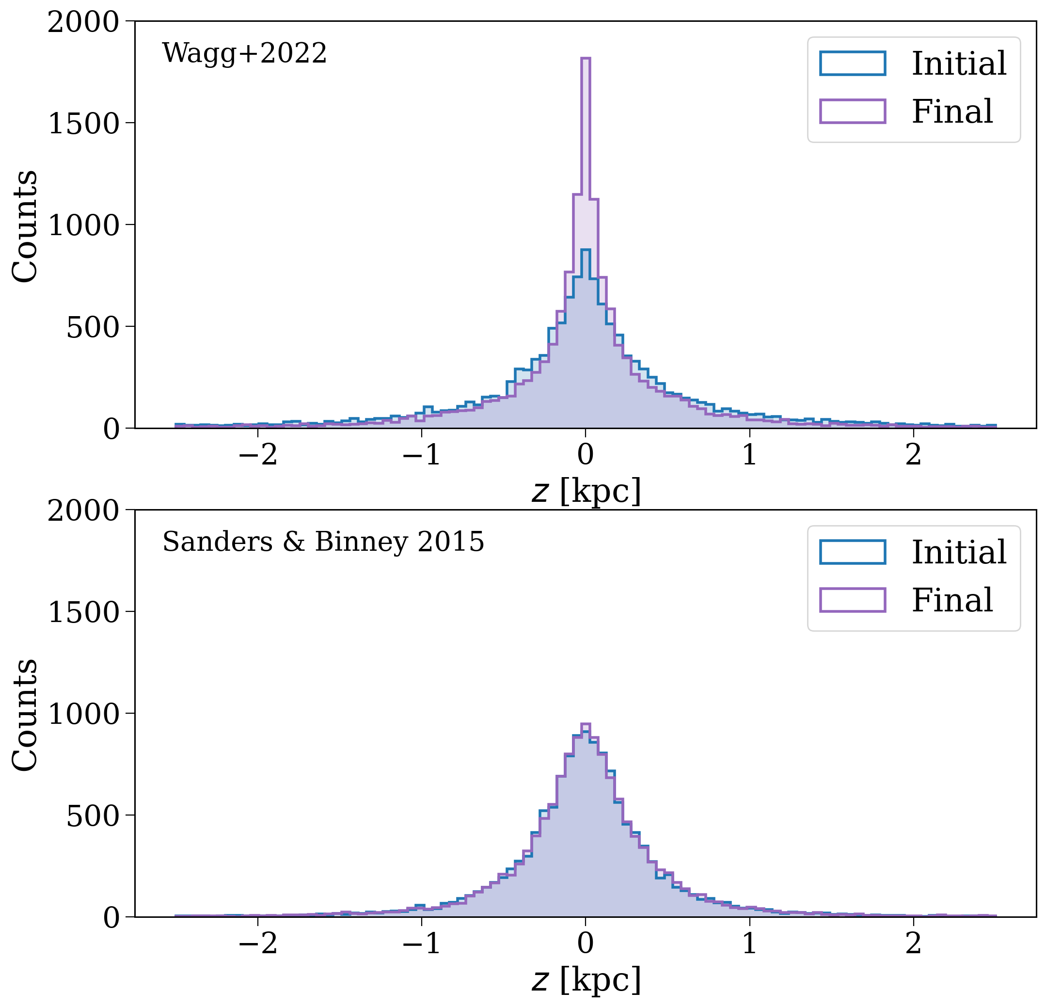
Aha! So the non-distribution function based SFH (Wagg+2022) clearly shows that the stars become more concentrated towards the galactic centre over time. Whereas the Sanders & Binney (2015) model is in steady-state and the two distributions are pretty much indistinguishable.

Wrap-up

And that’s all for this tutorial! You should now have a good understanding of how to use distribution function based star formation histories in cogsworth, and why they can be useful for generating more realistic stellar populations.

Note

This tutorial was generated from a Jupyter notebook that can be found here.