
Re-running for more detailed output#
Once you’ve selected a specific subpopulation you might need more detailed timestep output either in terms of the stellar or galactic evolution. In this tutorial we’ll go through how you can re-run a subpopulation to get more detailed output.
Learning Goals#
By the end of this tutorial you should know how to:
Choose
bcmconditions forCOSMICsimulationsApply
bcmconditions to a (sub)PopulationAdjust the orbit integration timestep size
If you’re not already familiar with selecting out subpopulations you may wish to check out this tutorial.
[1]:
import cogsworth
import matplotlib.pyplot as plt
import numpy as np
import pandas as pd
import astropy.units as u
[2]:
# this all just makes plots look nice
%config InlineBackend.figure_format = 'retina'

plt.rc('font', family='serif')
plt.rcParams['text.usetex'] = False
fs = 24

# update various fontsizes to match
params = {'figure.figsize': (12, 8),
          'legend.fontsize': fs,
          'axes.labelsize': fs,
          'xtick.labelsize': 0.9 * fs,
          'ytick.labelsize': 0.9 * fs,
          'axes.linewidth': 1.1,
          'xtick.major.size': 7,
          'xtick.minor.size': 4,
          'ytick.major.size': 7,
          'ytick.minor.size': 4}
plt.rcParams.update(params)
pd.options.display.max_columns = 999
Run a population to find a potential X-ray binary#
First let’s make a population and try to get a source that has a star transferring mass onto a compact object at some point.
[3]:
# keep making populations until we get at least one XRB
xrb_nums = []
while len(xrb_nums) == 0:
    # preferentially sample higher mass stars to get compact objects
    p = cogsworth.pop.Population(500, final_kstar1=[13, 14], use_default_BSE_settings=True)

    # we only need the stellar evolution for this case
    p.sample_initial_galaxy()
    p.sample_initial_binaries()
    p.perform_stellar_evolution()

    # find any stars with a compact object where the other star is overflowing its Roche lobe
    xrb_condition = ((p.bpp["kstar_1"].isin([13, 14]) & (p.bpp["RRLO_2"] >= 1)) |
                     (p.bpp["kstar_2"].isin([13, 14]) & (p.bpp["RRLO_1"] >= 1)))
    maybe_xrb_nums = p.bpp[xrb_condition]["bin_num"].unique()

    # find the binaries that have experienced a common envelope or merged
    ce_nums = p.bpp[p.bpp["evol_type"] == 7]["bin_num"].unique()
    merged_nums = p.bin_nums[p.final_bpp["sep"] == 0]
    xrb_nums = np.setdiff1d(maybe_xrb_nums, np.union1d(ce_nums, merged_nums))
Inspect our potential XRB#
Now let’s take a look at the evolution table for a random one of our XRBs.
[4]:
random_xrb = np.random.choice(xrb_nums)
p.bpp.loc[random_xrb]
[4]:
| tphys | mass_1 | mass_2 | kstar_1 | kstar_2 | sep | porb | ecc | RRLO_1 | RRLO_2 | evol_type | aj_1 | aj_2 | tms_1 | tms_2 | massc_he_layer_1 | massc_he_layer_2 | massc_co_layer_1 | massc_co_layer_2 | rad_1 | rad_2 | mass0_1 | mass0_2 | lum_1 | lum_2 | teff_1 | teff_2 | radc_1 | radc_2 | menv_1 | menv_2 | renv_1 | renv_2 | omega_spin_1 | omega_spin_2 | B_1 | B_2 | bacc_1 | bacc_2 | tacc_1 | tacc_2 | epoch_1 | epoch_2 | bhspin_1 | bhspin_2 | bin_num | |
|---|---|---|---|---|---|---|---|---|---|---|---|---|---|---|---|---|---|---|---|---|---|---|---|---|---|---|---|---|---|---|---|---|---|---|---|---|---|---|---|---|---|---|---|---|---|---|
| 284 | 0.000000 | 68.432984 | 32.322987 | 1 | 1 | 1354.551310 | 575.612151 | 0.178541 | 2.150881e-02 | 0.019301 | 1 | 0.000000 | 0.000000 | 3.895800e+00 | 6.050651e+00 | 0.000000 | 0.000000 | 0.000000 | 0.000000 | 10.651974 | 6.791114 | 68.432984 | 32.322987 | 6.291428e+05 | 1.337686e+05 | 50031.309993 | 42548.829216 | 0.000000 | 0.000000 | 1.000000e-10 | 1.000000e-10 | 1.000000e-10 | 1.000000e-10 | 9.423868e+02 | 1.517924e+03 | 0.0 | 0.0 | 0.0 | 0.0 | 0.0 | 0.0 | 0.000000 | 0.000000 | 0.0 | 0.0 | 284 |
| 284 | 4.004851 | 58.114616 | 31.478397 | 2 | 1 | 1522.717155 | 727.551853 | 0.178510 | 6.391345e-02 | 0.025409 | 2 | 4.174279 | 4.056045 | 4.174279e+00 | 6.185002e+00 | 23.185659 | 0.000000 | 0.000000 | 0.000000 | 34.608483 | 10.402299 | 58.114616 | 31.478397 | 1.114242e+06 | 2.052907e+05 | 32020.141959 | 38264.607022 | 1.565623 | 0.000000 | 1.000000e-10 | 1.000000e-10 | 1.000000e-10 | 1.000000e-10 | 4.074314e+01 | 5.244876e+02 | 0.0 | 0.0 | 0.0 | 0.0 | 0.0 | 0.0 | -0.169428 | -0.051194 | 0.0 | 0.0 | 284 |
| 284 | 4.008187 | 23.592003 | 32.910293 | 7 | 1 | 2207.554674 | 1599.213014 | 0.170933 | 2.466526e-03 | 0.014367 | 2 | 0.000000 | 3.913473 | 3.884565e-01 | 5.962596e+00 | 23.592003 | 0.000000 | 0.000000 | 0.000000 | 1.582219 | 10.729453 | 23.592003 | 32.910293 | 6.297103e+05 | 2.269043e+05 | 129843.906805 | 38631.494869 | 0.000000 | 0.000000 | 1.000000e-10 | 1.000000e-10 | 1.000000e-10 | 1.000000e-10 | 3.211439e-04 | 4.758087e+02 | 0.0 | 0.0 | 0.0 | 0.0 | 0.0 | 0.0 | 4.008187 | 0.094714 | 0.0 | 0.0 | 284 |
| 284 | 4.430819 | 17.147537 | 32.736217 | 8 | 1 | 2500.468808 | 2051.751492 | 0.170933 | 1.936963e-03 | 0.012947 | 2 | 0.462930 | 4.353873 | 4.629294e-01 | 5.988258e+00 | 4.363785 | 0.000000 | 12.783752 | 0.000000 | 1.303220 | 11.698923 | 17.147537 | 32.736217 | 5.429688e+05 | 2.407797e+05 | 137865.150135 | 37549.281094 | 0.000070 | 0.000000 | 1.000000e-10 | 1.000000e-10 | 1.000000e-10 | 1.000000e-10 | 3.773978e-02 | 3.838094e+02 | 0.0 | 0.0 | 0.0 | 0.0 | 0.0 | 0.0 | 3.967890 | 0.076946 | 0.0 | 0.0 | 284 |
| 284 | 4.433547 | 17.110553 | 32.735038 | 8 | 1 | 2502.383511 | 2054.894777 | 0.170933 | 1.936963e-03 | 0.012947 | 15 | 0.465657 | 4.356728 | 4.629294e-01 | 5.988433e+00 | 4.205507 | 0.000000 | 12.905046 | 0.000000 | 1.316028 | 11.706203 | 17.147537 | 32.735038 | 5.692211e+05 | 2.408737e+05 | 138821.688256 | 37541.266272 | 0.000070 | 0.000000 | 1.000000e-10 | 1.000000e-10 | 1.000000e-10 | 1.000000e-10 | 1.607338e+06 | 3.832233e+02 | 0.0 | 0.0 | 0.0 | 0.0 | 0.0 | 0.0 | 3.967890 | 0.076819 | 0.0 | 0.0 | 284 |
| 284 | 4.433547 | 16.610553 | 32.735038 | 14 | 1 | 2523.647500 | 2091.659661 | 0.166265 | 1.039600e-07 | 0.012682 | 2 | 0.000000 | 4.356728 | 4.629294e-01 | 5.988433e+00 | 0.000000 | 0.000000 | 0.000000 | 0.000000 | 0.000070 | 11.706204 | 17.147537 | 32.735038 | 1.000000e-10 | 2.408737e+05 | 2184.714229 | 37541.264968 | 0.000070 | 0.000000 | 1.000000e-10 | 1.000000e-10 | 1.000000e-10 | 1.000000e-10 | 1.607338e+06 | 3.832232e+02 | 0.0 | 0.0 | 0.0 | 0.0 | 0.0 | 0.0 | 4.433547 | 0.076819 | 0.0 | 0.0 | 284 |
| 284 | 6.080704 | 16.610642 | 32.008187 | 14 | 2 | 2560.773475 | 2153.905557 | 0.166264 | 1.018780e-07 | 0.019968 | 2 | 1.647157 | 6.099626 | 1.000000e+10 | 6.099625e+00 | 0.000000 | 10.360793 | 0.000000 | 0.000000 | 0.000070 | 18.616563 | 17.147537 | 32.008187 | 1.000000e-10 | 3.407618e+05 | 2184.708392 | 32466.284813 | 0.000070 | 0.957364 | 1.000000e-10 | 1.000000e-10 | 1.000000e-10 | 1.000000e-10 | 2.806232e+08 | 1.870100e+02 | 0.0 | 0.0 | 0.0 | 0.0 | 0.0 | 0.0 | 4.433547 | -0.018922 | 0.0 | 0.0 | 284 |
| 284 | 6.088432 | 16.611136 | 31.979980 | 14 | 4 | 2562.077588 | 2156.165712 | 0.166260 | 1.018054e-07 | 0.563961 | 2 | 1.654885 | 6.107354 | 1.000000e+10 | 6.099625e+00 | 0.000000 | 10.567995 | 0.000000 | 0.000000 | 0.000070 | 525.977685 | 17.147537 | 32.008187 | 1.000000e-10 | 3.764246e+05 | 2184.675862 | 6261.890090 | 0.000070 | 0.969099 | 1.000000e-10 | 1.000000e-10 | 1.000000e-10 | 1.000000e-10 | 9.010750e+08 | 1.762017e-01 | 0.0 | 0.0 | 0.0 | 0.0 | 0.0 | 0.0 | 4.433547 | -0.018922 | 0.0 | 0.0 | 284 |
| 284 | 6.137317 | 16.643037 | 31.345194 | 14 | 4 | 2155.013732 | 1673.708606 | 0.000000 | 1.005523e-07 | 1.000003 | 3 | 1.703770 | 6.156239 | 1.000000e+10 | 6.099625e+00 | 0.000000 | 10.773859 | 0.000000 | 0.000000 | 0.000071 | 936.693801 | 17.147537 | 32.008187 | 1.000000e-10 | 3.824015e+05 | 2182.581085 | 4710.865148 | 0.000071 | 0.994073 | 1.000000e-10 | 4.088808e-04 | 1.000000e-10 | 6.247699e+01 | 2.849011e+10 | 1.371129e+00 | 0.0 | 0.0 | 0.0 | 0.0 | 0.0 | 0.0 | 4.433547 | -0.018922 | 0.0 | 0.0 | 284 |
| 284 | 6.621218 | 19.716657 | 12.936438 | 14 | 4 | 2425.758062 | 2423.155061 | 0.000000 | 8.287052e-08 | 0.751796 | 4 | 2.187671 | 6.640140 | 1.000000e+10 | 6.099625e+00 | 0.000000 | 12.811668 | 0.000000 | 0.000000 | 0.000084 | 625.667982 | 17.147537 | 32.008187 | 1.000000e-10 | 4.460909e+05 | 2005.256986 | 5990.367703 | 0.000084 | 1.167696 | 1.000000e-10 | 1.000000e-10 | 1.000000e-10 | 1.000000e-10 | 1.147643e+11 | 2.247050e+00 | 0.0 | 0.0 | 0.0 | 0.0 | 0.0 | 0.0 | 4.433547 | -0.018922 | 0.0 | 0.0 | 284 |
| 284 | 6.635357 | 19.725034 | 12.871191 | 14 | 7 | 2427.934555 | 2428.532783 | 0.000000 | 8.273486e-08 | 0.001398 | 2 | 2.201809 | 0.484999 | 1.000000e+10 | 5.481426e-01 | 0.000000 | 4.751005 | 0.000000 | 8.120186 | 0.000084 | 1.162799 | 17.147537 | 12.871191 | 1.000000e-10 | 3.144633e+05 | 2004.831131 | 127323.825971 | 0.000084 | 0.000084 | 1.000000e-10 | 1.000000e-10 | 1.000000e-10 | 1.000000e-10 | 1.148816e+11 | 2.075600e-10 | 0.0 | 0.0 | 0.0 | 0.0 | 0.0 | 0.0 | 4.433547 | 6.150357 | 0.0 | 0.0 | 284 |
| 284 | 6.699062 | 19.725037 | 12.507274 | 14 | 8 | 2455.348739 | 2483.683286 | 0.000000 | 8.131488e-08 | 0.001286 | 2 | 2.265515 | 0.557956 | 1.000000e+10 | 5.579554e-01 | 0.000000 | 3.633483 | 0.000000 | 8.873791 | 0.000084 | 1.074704 | 17.147537 | 12.507274 | 1.000000e-10 | 3.091389e+05 | 2004.831018 | 131875.355745 | 0.000084 | 0.000070 | 1.000000e-10 | 1.000000e-10 | 1.000000e-10 | 1.000000e-10 | 1.148816e+11 | 2.382864e-10 | 0.0 | 0.0 | 0.0 | 0.0 | 0.0 | 0.0 | 4.433547 | 6.141107 | 0.0 | 0.0 | 284 |
| 284 | 6.714987 | 19.725037 | 12.399790 | 14 | 8 | 2463.565054 | 2500.332761 | 0.000000 | 8.131488e-08 | 0.001286 | 16 | 2.281440 | 0.573870 | 1.000000e+10 | 5.579554e-01 | 0.000000 | 3.081667 | 0.000000 | 9.318123 | 0.000084 | 1.145790 | 17.147537 | 12.507274 | 1.000000e-10 | 3.946136e+05 | 2004.830985 | 135756.346292 | 0.000084 | 0.000070 | 1.000000e-10 | 1.000000e-10 | 1.000000e-10 | 1.000000e-10 | 1.148816e+11 | 2.997945e-02 | 0.0 | 0.0 | 0.0 | 0.0 | 0.0 | 0.0 | 4.433547 | 6.141107 | 0.0 | 0.0 | 284 |
| 284 | 6.714987 | 19.725037 | 9.595666 | 14 | 14 | -1.000000 | -1.000000 | -1.000000 | 0.000000e+00 | -2.000000 | 11 | 2.281440 | 0.573870 | 1.000000e+10 | 5.579554e-01 | 0.000000 | 3.081667 | 0.000000 | 9.318123 | 0.000084 | 1.145790 | 17.147537 | 12.507274 | 1.000000e-10 | 3.946136e+05 | 2004.830985 | 135756.346292 | 0.000084 | 0.000070 | 1.000000e-10 | 1.000000e-10 | 1.000000e-10 | 1.000000e-10 | 1.148816e+11 | 2.997945e-02 | 0.0 | 0.0 | 0.0 | 0.0 | 0.0 | 0.0 | 4.433547 | 6.714987 | 0.0 | 0.0 | 284 |
| 284 | 11587.184534 | 19.725037 | 9.595666 | 14 | 14 | -1.000000 | -1.000000 | -1.000000 | 1.000000e-04 | 0.000100 | 10 | 11582.750987 | 11580.469548 | 1.000000e+10 | 1.000000e+10 | 0.000000 | 3.081667 | 0.000000 | 9.318123 | 0.000084 | 0.000041 | 17.147537 | 12.507274 | 1.000000e-10 | 1.000000e-10 | 2004.830985 | 2874.412757 | 0.000084 | 0.000041 | 1.000000e-10 | 1.000000e-10 | 1.000000e-10 | 1.000000e-10 | 1.148816e+11 | 2.000000e+08 | 0.0 | 0.0 | 0.0 | 0.0 | 0.0 | 0.0 | 4.433547 | 6.714987 | 0.0 | 0.0 | 284 |
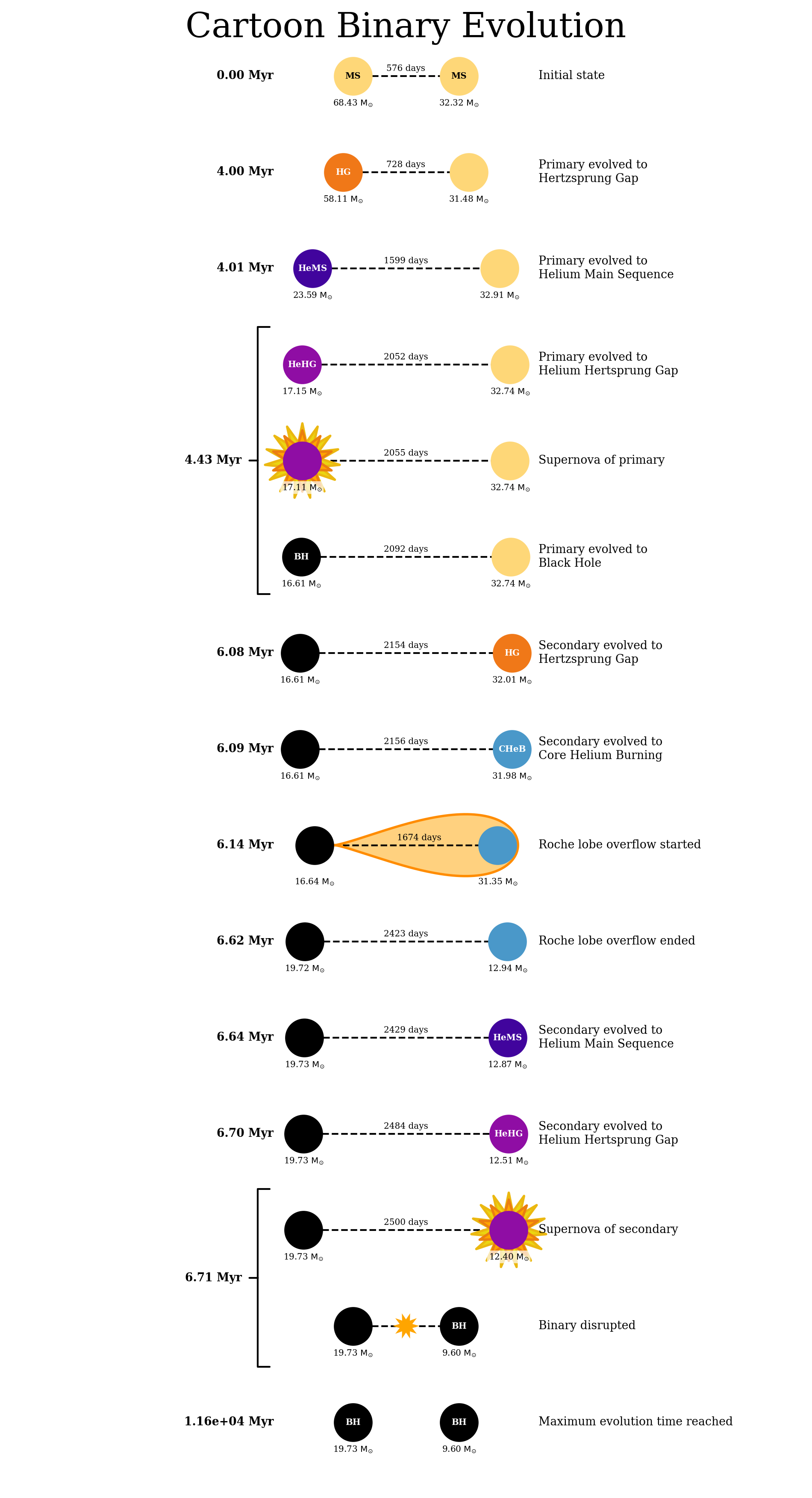
That’s a lot of numbers, let’s use cogsworth to turn this into a plot to make things easier.
[5]:
p.plot_cartoon_binary(random_xrb)
[5]:
(<Figure size 1200x2250 with 1 Axes>, <Axes: >)
Re-run for more detail#
Okay so we can see that this random binary had some mass transfer onto a compact object, but what was the mass transfer rate over time? Exactly how long did it last? We can’t really see that currently. Luckily COSMIC makes it very easy to re-run this binary with more detail.
To start let’s make a population with this binary all by itself.
[6]:
xrb = p[int(random_xrb)]
Now let’s overwrite the bcm_timestep_conditions for this population and re-run the stellar evolution.
[7]:
# these conditions say "one star is a NS/BH, the other is a star that is overflowing its Roche lobe"
# they then specify dtp=0.0 which means "give me every timestep you computed"
# you could set this to a value in Myr to get fewer timesteps
xrb.bcm_timestep_conditions = [
    ['kstar_1>=13', 'kstar_2<10', 'RRLO_2>=1', 'dtp=0.0'],
    ['kstar_2>=13', 'kstar_1<10', 'RRLO_1>=1', 'dtp=0.0'],
]

# we can also erase our BSE_settings now that they are stored in the initial_binaries table
xrb.BSE_settings = {}

xrb.perform_stellar_evolution()
And with that done we now have a new p.bcm table that includes all of the details of the mass transfer onto the black hole
[8]:
xrb.bcm
[8]:
| tphys | kstar_1 | mass0_1 | mass_1 | lum_1 | rad_1 | teff_1 | massc_he_layer_1 | massc_co_layer_1 | radc_1 | menv_1 | renv_1 | epoch_1 | omega_spin_1 | deltam_1 | RRLO_1 | kstar_2 | mass0_2 | mass_2 | lum_2 | rad_2 | teff_2 | massc_he_layer_2 | massc_co_layer_2 | radc_2 | menv_2 | renv_2 | epoch_2 | omega_spin_2 | deltam_2 | RRLO_2 | porb | sep | ecc | B_1 | B_2 | SN_1 | SN_2 | bin_state | merger_type | bin_num | |
|---|---|---|---|---|---|---|---|---|---|---|---|---|---|---|---|---|---|---|---|---|---|---|---|---|---|---|---|---|---|---|---|---|---|---|---|---|---|---|---|---|---|
| 284 | 0.000000 | 1 | 68.432984 | 68.432984 | 6.291428e+05 | 10.651974 | 50031.309993 | 0.0 | 0.0 | 0.000000 | 1.000000e-10 | 1.000000e-10 | 0.000000 | 9.423868e+02 | 0.000000 | 2.150881e-02 | 1 | 32.322987 | 32.322987 | 1.337686e+05 | 6.791114 | 42548.829216 | 0.000000 | 0.000000 | 0.000000 | 1.000000e-10 | 1.000000e-10 | 0.000000 | 1.517924e+03 | 0.000000 | 0.019301 | 575.612151 | 1354.551310 | 0.178541 | 0.0 | 0.0 | 0 | 0 | 0 | -001 | 284 |
| 284 | 6.137317 | 14 | 17.147537 | 16.643037 | 1.000000e-10 | 0.000071 | 2182.581085 | 0.0 | 0.0 | 0.000071 | 1.000000e-10 | 1.000000e-10 | 4.433547 | 2.849011e+10 | 0.000000 | 1.005523e-07 | 4 | 32.008187 | 31.345194 | 3.824015e+05 | 936.693801 | 4710.865148 | 10.773859 | 0.000000 | 0.994073 | 4.088808e-04 | 6.247699e+01 | -0.018922 | 1.371129e+00 | 0.000000 | 1.000003 | 1673.708606 | 2155.013732 | 0.000000 | 0.0 | 0.0 | 1 | 0 | 0 | -001 | 284 |
| 284 | 6.137321 | 14 | 17.147537 | 16.643044 | 1.000000e-10 | 0.000071 | 2182.580672 | 0.0 | 0.0 | 0.000071 | 1.000000e-10 | 1.000000e-10 | 4.433547 | 2.863506e+10 | 0.000002 | 1.005522e-07 | 4 | 32.008187 | 31.345125 | 3.824019e+05 | 936.817743 | 4710.554919 | 10.773875 | 0.000000 | 0.994074 | 4.143226e-04 | 6.269220e+01 | -0.018922 | 1.371112e+00 | -0.000019 | 1.000135 | 1673.711080 | 2155.014918 | 0.000000 | 0.0 | 0.0 | 1 | 0 | 0 | -001 | 284 |
| 284 | 6.137328 | 14 | 17.147537 | 16.643056 | 1.000000e-10 | 0.000071 | 2182.579847 | 0.0 | 0.0 | 0.000071 | 1.000000e-10 | 1.000000e-10 | 4.433547 | 2.892494e+10 | 0.000002 | 1.005520e-07 | 4 | 32.008187 | 31.344987 | 3.824028e+05 | 937.065734 | 4709.934376 | 10.773906 | 0.000000 | 0.994078 | 4.253834e-04 | 6.312334e+01 | -0.018922 | 1.371062e+00 | -0.000019 | 1.000400 | 1673.716029 | 2155.017289 | 0.000000 | 0.0 | 0.0 | 1 | 0 | 0 | -001 | 284 |
| 284 | 6.137343 | 14 | 17.147537 | 16.643082 | 1.000000e-10 | 0.000071 | 2182.578196 | 0.0 | 0.0 | 0.000071 | 1.000000e-10 | 1.000000e-10 | 4.433547 | 2.950469e+10 | 0.000002 | 1.005517e-07 | 4 | 32.008187 | 31.344711 | 3.824047e+05 | 937.562144 | 4708.692958 | 10.773969 | 0.000000 | 0.994086 | 4.482288e-04 | 6.398848e+01 | -0.018922 | 1.370962e+00 | -0.000019 | 1.000930 | 1673.725927 | 2155.022031 | 0.000000 | 0.0 | 0.0 | 1 | 0 | 0 | -001 | 284 |
| ... | ... | ... | ... | ... | ... | ... | ... | ... | ... | ... | ... | ... | ... | ... | ... | ... | ... | ... | ... | ... | ... | ... | ... | ... | ... | ... | ... | ... | ... | ... | ... | ... | ... | ... | ... | ... | ... | ... | ... | ... | ... |
| 284 | 6.615655 | 14 | 17.147537 | 19.682717 | 1.000000e-10 | 0.000083 | 2006.985129 | 0.0 | 0.0 | 0.000083 | 1.000000e-10 | 1.000000e-10 | 4.433547 | 1.151000e+11 | 0.000006 | 8.306739e-08 | 4 | 32.008187 | 13.077226 | 4.460617e+05 | 1485.377137 | 3887.764674 | 12.788240 | 0.000000 | 1.169206 | 1.000000e-10 | 1.000000e-10 | -0.018922 | 4.979042e-15 | -0.000037 | 1.781918 | 2414.047591 | 2422.312438 | 0.000000 | 0.0 | 0.0 | 1 | 0 | 0 | -001 | 284 |
| 284 | 6.617509 | 14 | 17.147537 | 19.694038 | 1.000000e-10 | 0.000084 | 2006.408224 | 0.0 | 0.0 | 0.000084 | 1.000000e-10 | 1.000000e-10 | 4.433547 | 1.149016e+11 | 0.000006 | 8.294392e-08 | 4 | 32.008187 | 13.017387 | 4.462439e+05 | 1319.796351 | 4124.860110 | 12.796049 | 0.000000 | 1.168728 | 1.000000e-10 | 1.000000e-10 | -0.018922 | 1.079896e+00 | -0.000032 | 1.583740 | 2419.324845 | 2424.643184 | 0.000000 | 0.0 | 0.0 | 1 | 0 | 0 | -001 | 284 |
| 284 | 6.619364 | 14 | 17.147537 | 19.705351 | 1.000000e-10 | 0.000084 | 2005.832178 | 0.0 | 0.0 | 0.000084 | 1.000000e-10 | 1.000000e-10 | 4.433547 | 1.149620e+11 | 0.000006 | 8.280819e-08 | 4 | 32.008187 | 12.970857 | 4.463097e+05 | 1035.159093 | 4657.738900 | 12.803859 | 0.000000 | 1.168224 | 1.000000e-10 | 1.000000e-10 | -0.018922 | 8.614461e-15 | -0.000025 | 1.241784 | 2425.449699 | 2427.861784 | 0.000000 | 0.0 | 0.0 | 1 | 0 | 0 | -001 | 284 |
| 284 | 6.621218 | 14 | 17.147537 | 19.716657 | 1.000000e-10 | 0.000084 | 2005.256986 | 0.0 | 0.0 | 0.000084 | 1.000000e-10 | 1.000000e-10 | 4.433547 | 1.147643e+11 | 0.000006 | 8.287052e-08 | 4 | 32.008187 | 12.936438 | 4.460909e+05 | 625.667982 | 5990.367703 | 12.811668 | 0.000000 | 1.167696 | 1.000000e-10 | 1.000000e-10 | -0.018922 | 2.247050e+00 | -0.000019 | 0.751796 | 2423.155061 | 2425.758062 | 0.000000 | 0.0 | 0.0 | 1 | 0 | 0 | -001 | 284 |
| 284 | 11587.184534 | 14 | 17.147537 | 19.725037 | 1.000000e-10 | 0.000084 | 2004.830985 | 0.0 | 0.0 | 0.000084 | 1.000000e-10 | 1.000000e-10 | 4.433547 | 1.148816e+11 | 0.000000 | 1.000000e-04 | 14 | 12.507274 | 9.595666 | 1.000000e-10 | 0.000041 | 2874.412757 | 3.081667 | 9.318123 | 0.000041 | 1.000000e-10 | 1.000000e-10 | 6.714987 | 2.000000e+08 | 0.000000 | 0.000100 | -1.000000 | -1.000000 | -1.000000 | 0.0 | 0.0 | 1 | 1 | 2 | -001 | 284 |
290 rows × 41 columns
Plotting time!#
It’s everyone’s favourite moment: plotting time! Let’s see how the mass of both companions varies during the mass transfer and how the mass transfer efficiency changes.
[9]:
mt_rows = xrb.bcm[xrb.bcm["RRLO_2"] >= 1]
[10]:
fig, axes = plt.subplots(2, 1, figsize=(12, 18))

mt_time = (mt_rows["tphys"] - mt_rows["tphys"].min()) * 1000

axes[0].scatter(mt_time, mt_rows["mass_2"], color="tab:green")
axes[0].spines["left"].set_color("tab:green")
axes[0].set_ylabel(r"Donor Mass [$M_{\odot}$]", color="tab:green")
axes[0].tick_params(axis="y", colors="tab:green")
axes[0].set_xlabel("Time [kyr]")

right_ax = axes[0].twinx()
right_ax.scatter(mt_time, mt_rows["mass_1"], color="tab:purple")
right_ax.spines["right"].set_color("tab:purple")
right_ax.set_ylabel(r"Accretor (black hole) mass [$M_{\odot}$]", color="tab:purple")
right_ax.tick_params(axis="y", colors="tab:purple")

axes[1].scatter(mt_time, mt_rows["deltam_1"] / -mt_rows["deltam_2"])
axes[1].set_ylabel(r"Mass transfer efficiency")
axes[1].set_xlabel("Time [kyr]")

plt.show()
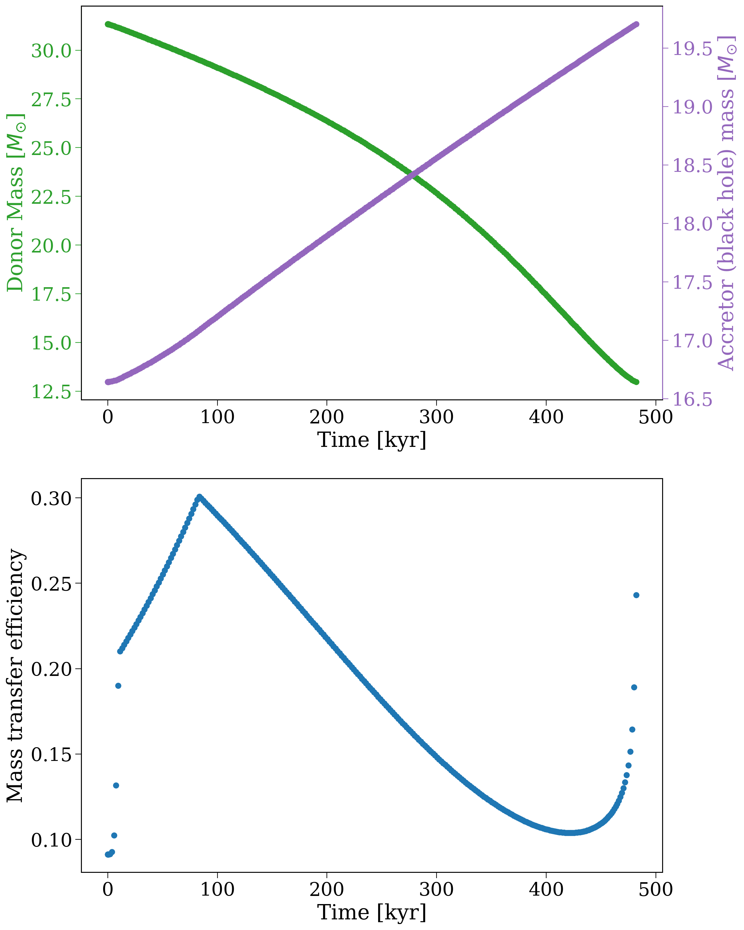
So you can see that the secondary transfers a lot of mass, but the black hole only accretes a very small fraction of it. You could imagine using this information to estimate the X-ray luminosity of the binary during this phase. But I’ll leave that as an exercise to the reader ;)
Wrap-up#
And now you know how to re-run your binaries in detail! You might want to try this yourself but for a different subpopulation, with different conditions! Keep reading for more fun cogsworth tutorials (disclaimer: fun not guaranteed…).
Note
This tutorial was generated from a Jupyter notebook that can be found here.