Exploring other star formation histories

In this tutorial we’ll discuss some of the other star formation histories available in the cogsworth.sfh module. For an introduction to this framework please checkout the Changing galactic star formation history models tutorial.

Learning Goals

By the end of this tutorial you should know how to:

• Use the simple disc star formation histories (BurstUniformDisc and ConstantUniformDisc) available and build upon them

• Apply the ConstantPlummerSphere SFH and modify it for your own needs

import cogsworth
import matplotlib.pyplot as plt
import numpy as np
import pandas as pd
import astropy.units as u

# this all just makes plots look nice
%config InlineBackend.figure_format = 'retina'

plt.rc('font', family='serif')
plt.rcParams['text.usetex'] = False
fs = 24

# update various fontsizes to match
params = {'figure.figsize': (12, 8),
          'legend.fontsize': fs,
          'axes.labelsize': fs,
          'xtick.labelsize': 0.9 * fs,
          'ytick.labelsize': 0.9 * fs,
          'axes.linewidth': 1.1,
          'xtick.major.size': 7,
          'xtick.minor.size': 4,
          'ytick.major.size': 7,
          'ytick.minor.size': 4}
plt.rcParams.update(params)
pd.options.display.max_columns = 999

Some simpler star formation histories

In an earlier tutorial (here), we explored the Wagg2022 class which attempts to model the history of the Milky Way in some detail. However, sometimes you may want to use a simpler model for the star formation history of your galaxy. We provide two simple disc SFHs that you can use out-of-the-box: BurstUniformDisc and ConstantUniformDisc. These classes both assume a disc-like spatial distribution of stars, a truly uniform cylinder, but have different temporal behaviour.

• BurstUniformDisc assumes that all stars are formed in a single burst at a specified time in the past.

• ConstantUniformDisc assumes that stars are formed at a constant rate over a specified time interval.

Let’s sample the same number of stars from each class with the exact same parameters and compare

burst = cogsworth.sfh.BurstUniformDisc(100000, t_burst=5*u.Gyr, z_max=3*u.kpc, R_max=15*u.kpc, Z_all=0.02)
constant = cogsworth.sfh.ConstantUniformDisc(100000, t_burst=5*u.Gyr, z_max=3*u.kpc, R_max=15*u.kpc, Z_all=0.02)

fig, ax = plt.subplots(1, 3, figsize=(30, 6))

ax[0].scatter(burst.x, burst.y, s=0.1, color='C0', label='BurstUniformDisc')
ax[0].scatter(constant.x, constant.y, s=0.1, color='C1', label='ConstantUniformDisc')
ax[0].set_xlabel('x [kpc]')
ax[0].set_ylabel('y [kpc]')
ax[0].set_aspect('equal')

ax[1].scatter(burst.x, burst.z, s=0.1, color='C0', label='BurstUniformDisc')
ax[1].scatter(constant.x, constant.z, s=0.1, color='C1', label='ConstantUniformDisc')
ax[1].set_xlabel('x [kpc]')
ax[1].set_ylabel('z [kpc]')
ax[1].set_aspect('equal')

ax[2].axvline(5, color='C0', lw=5)
ax[2].hist(constant.tau.to(u.Gyr).value, bins=np.linspace(0, 5, 100), alpha=0.7, color='C1', label='ConstantUniformDisc')
ax[2].set_xlabel('Lookback time [Gyr]')
ax[2].set_ylabel('Number of stars')

ax[1].legend(markerscale=50, fontsize=0.6 * fs, loc='lower center', bbox_to_anchor=(0.5, 1.0), ncol=2)

<matplotlib.legend.Legend at 0x13a194d50>

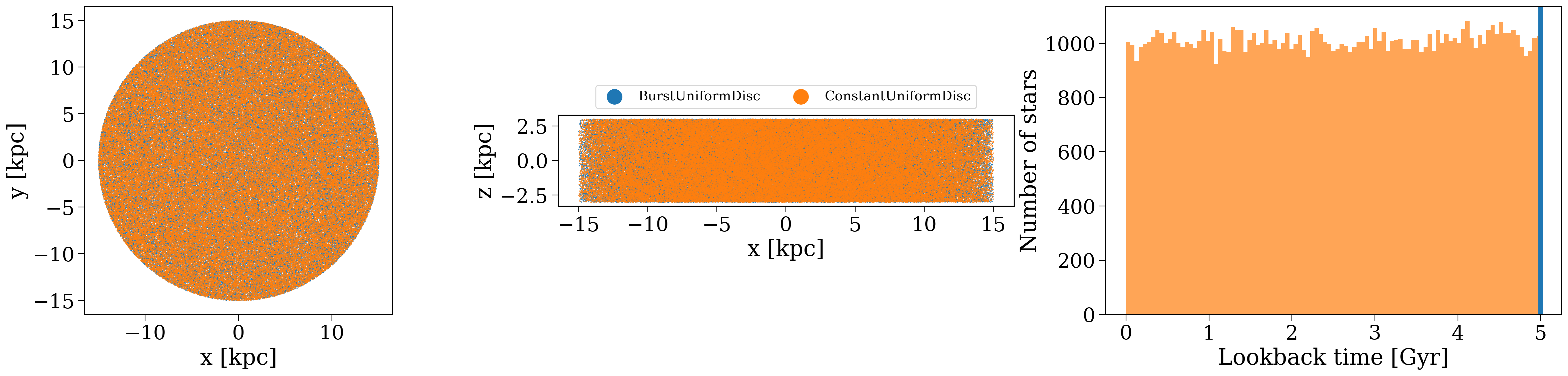
Spatially the distributions are identical, the difference is only in the lookback time plot.

Building upon the classes

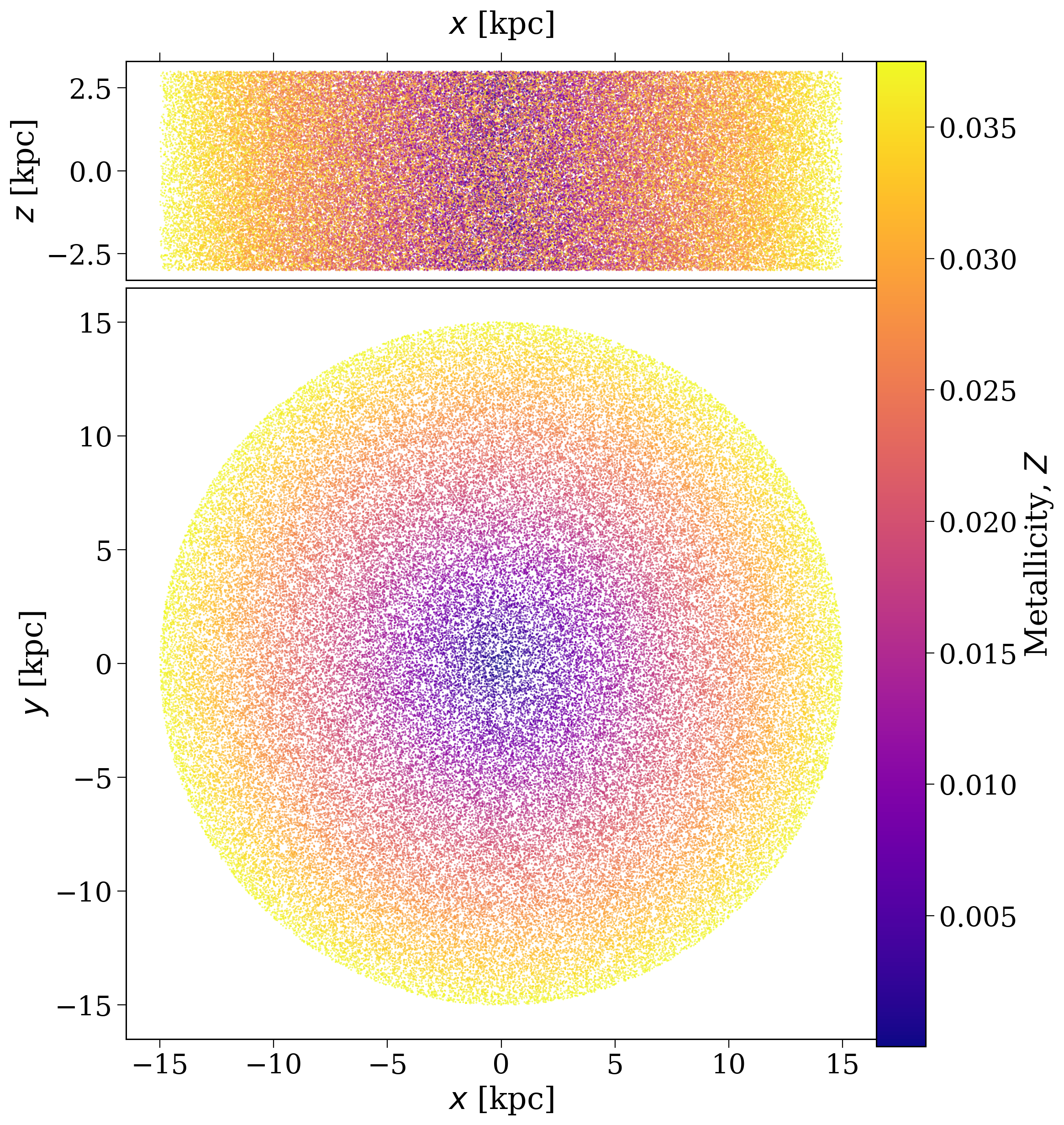
Now let’s say you want to build a constant uniform disc that had a linearly increasing metallicity with radius. You can easily subclass ConstantUniformDisc to do this:

class LinearMetallicityDisc(cogsworth.sfh.ConstantUniformDisc):
    def get_metallicity(self):
        """Linearly increasing metallicity with radius, starts at 0, solar at 8 kpc"""
        self._Z = self.rho.to(u.kpc).value * 0.02 / 8 * u.dimensionless_unscaled
        return self._Z

disc = LinearMetallicityDisc(100000, t_burst=5*u.Gyr, z_max=3*u.kpc, R_max=15*u.kpc)
disc.plot(cbar_norm=None)

(<Figure size 1247.5x1400 with 3 Axes>,
 array([<Axes: xlabel='$x$ [kpc]', ylabel='$z$ [kpc]'>,
        <Axes: xlabel='$x$ [kpc]', ylabel='$y$ [kpc]'>], dtype=object))

I’ll leave it as an exercise to you to consider how you could modify it to depend on the age as well!

Sampling from a Plummer sphere

The basics

Many star clusters and dwarf galaxies can be well modelled by a Plummer sphere spatial distribution. cogsworth provides the ConstantPlummerSphere class to sample stars from such a distribution with a constant star formation history and fixed metallicity. Importantly, this class samples velocities consistently as well using the Plummer potential, so that the resulting population is in equilibrium. You can learn more about sampling from more general distribution-function based in the next tutorial.

Here’s an example of how to use it:

It looks much like a normal star formation history call but now we also provide a Plummer mass of \(10^{10} M_\odot\) and a scale radius of 5 kpc.

plummer = cogsworth.sfh.ConstantPlummerSphere(
    size=100000,
    tau_min=0*u.Gyr,
    tau_max=10*u.Gyr,
    Z_all=0.02,
    M=1e10*u.Msun,
    a=5.0*u.kpc,
)

Now let’s make those same plots as earlier.

fig, ax = plt.subplots(1, 3, figsize=(30, 6))

ax[0].scatter(plummer.x, plummer.y, s=0.1, color='C0', label='BurstUniformDisc')
ax[0].set_xlabel('x [kpc]')
ax[0].set_ylabel('y [kpc]')
ax[0].set_aspect('equal')

ax[1].scatter(plummer.x, plummer.z, s=0.1, color='C0', label='BurstUniformDisc')
ax[1].set_xlabel('x [kpc]')
ax[1].set_ylabel('z [kpc]')
ax[1].set_aspect('equal')

ax[2].hist(plummer.tau.to(u.Gyr).value, bins=np.linspace(0, 5, 100), alpha=0.7, color='C1', label='ConstantUniformDisc')
ax[2].set_xlabel('Lookback time [Gyr]')
ax[2].set_ylabel('Number of stars')

Text(0, 0.5, 'Number of stars')

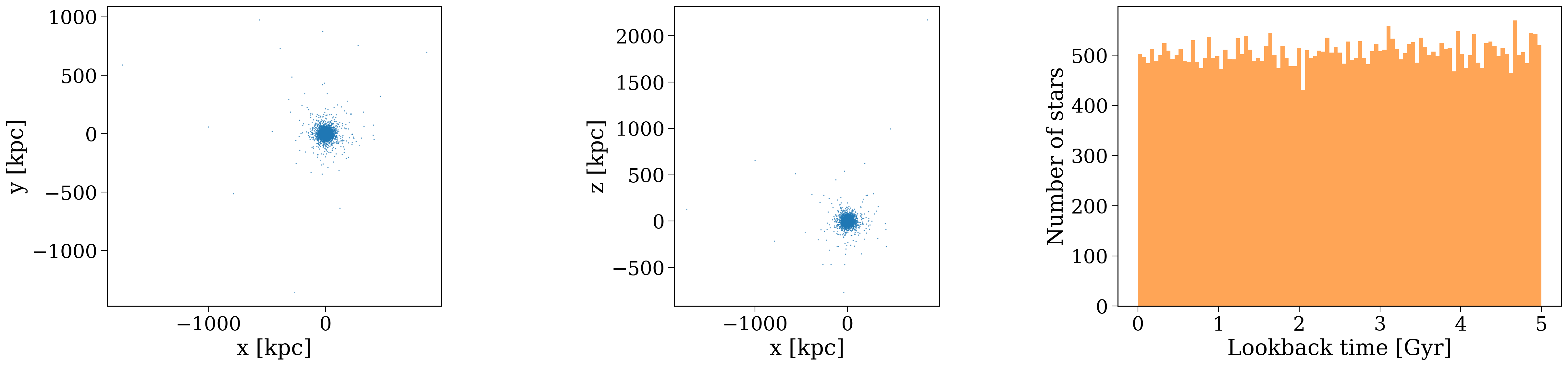
Hmm, well as you can see, if we sample 100,000 points, given the infinite extent of a Plummer sphere, you can end up with some very far out points, even with only a scale radius of 5 kpc.

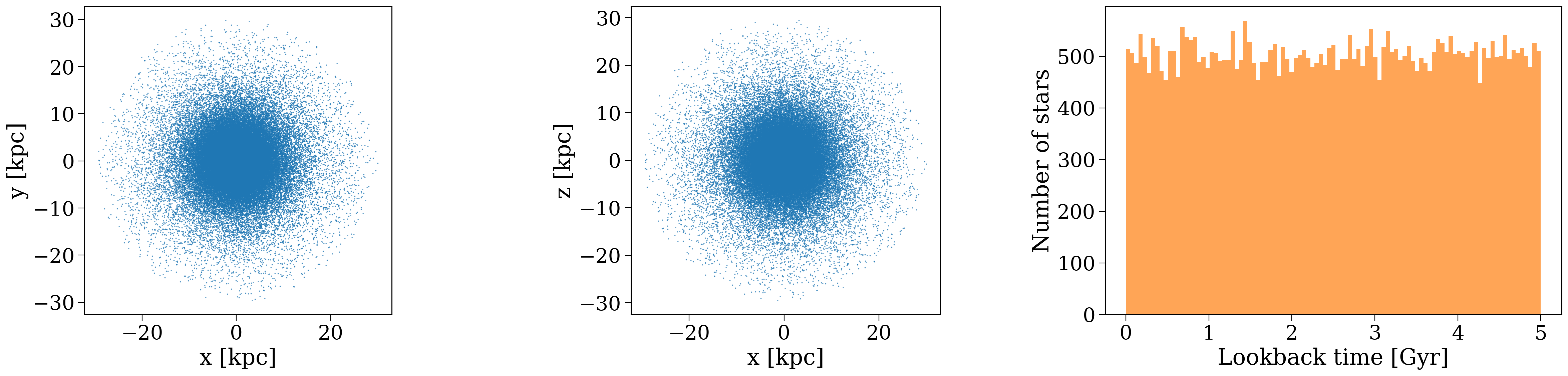
Truncation

One can therefore truncate the radial distribution at a given value. Let’s use 30 kpc for instance, such that anything beyond this gets resampled. Note that this makes the velocities not entirely self-consistent now since we exclude part of the distribution, but this is only a small correction.

plummer_trunc = cogsworth.sfh.ConstantPlummerSphere(
    size=100000,
    tau_min=0*u.Gyr,
    tau_max=10*u.Gyr,
    Z_all=0.02,
    M=1e10*u.Msun,
    a=5.0*u.kpc,
    r_trunc=30*u.kpc        # <-- THIS IS THE CHANGE
)

fig, ax = plt.subplots(1, 3, figsize=(30, 6))

ax[0].scatter(plummer_trunc.x, plummer_trunc.y, s=0.1, color='C0', label='BurstUniformDisc')
ax[0].set_xlabel('x [kpc]')
ax[0].set_ylabel('y [kpc]')
ax[0].set_aspect('equal')

ax[1].scatter(plummer_trunc.x, plummer_trunc.z, s=0.1, color='C0', label='BurstUniformDisc')
ax[1].set_xlabel('x [kpc]')
ax[1].set_ylabel('z [kpc]')
ax[1].set_aspect('equal')

ax[2].hist(plummer_trunc.tau.to(u.Gyr).value, bins=np.linspace(0, 5, 100), alpha=0.7, color='C1', label='ConstantUniformDisc')
ax[2].set_xlabel('Lookback time [Gyr]')
ax[2].set_ylabel('Number of stars')

Text(0, 0.5, 'Number of stars')

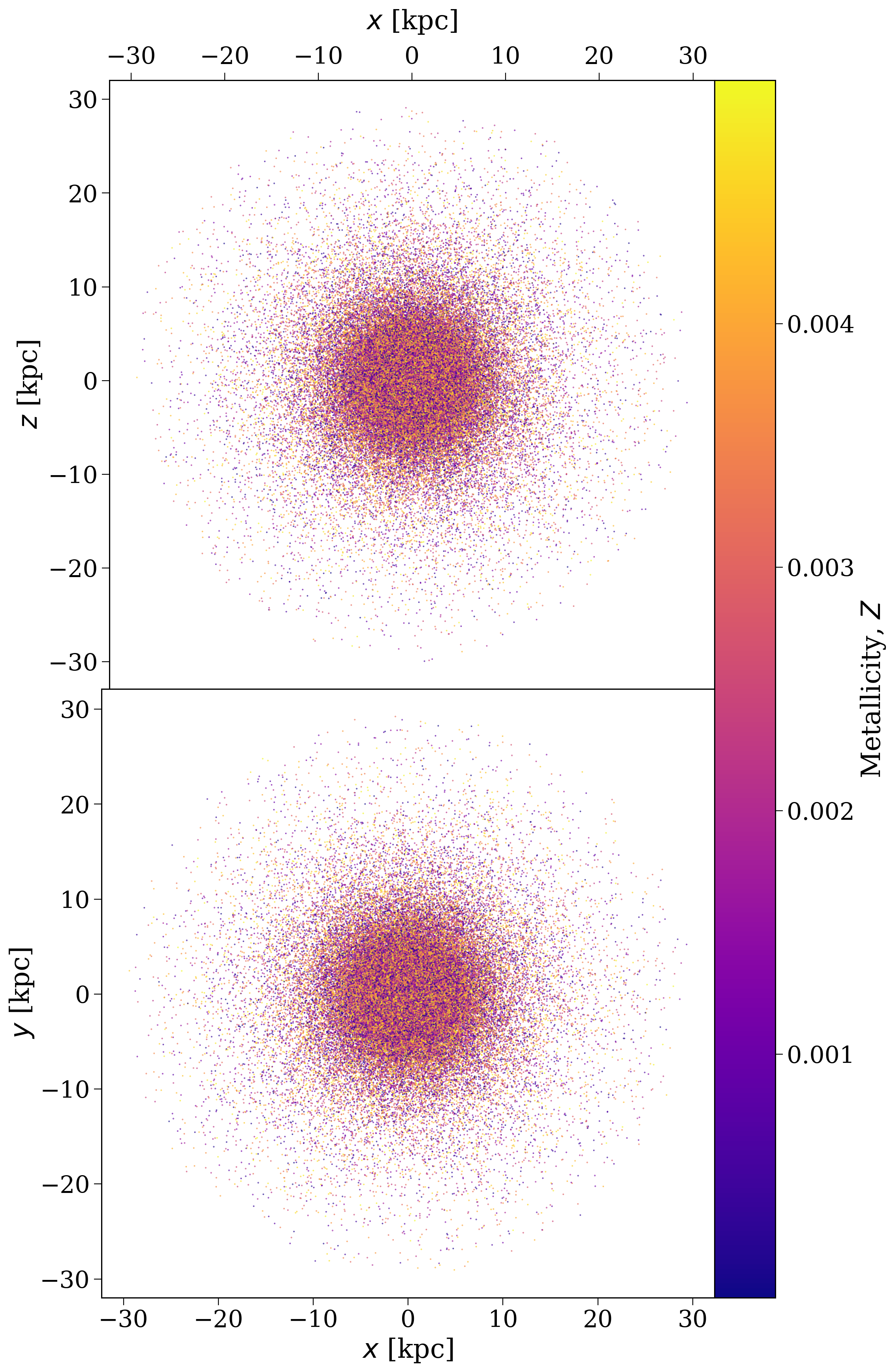
Add metallicity evolution

Perhaps you might also want your metallicity growing as a function of time, why not subclass it!

class LinearZTimePlummer(cogsworth.sfh.ConstantPlummerSphere):
    def __init__(self, Z_min=0, Z_scale=0.0025, **kwargs):
        self.Z_min = Z_min
        self.Z_scale = Z_scale
        super().__init__(**kwargs)

    def get_metallicity(self):
        """Linearly increasing metallicity with time"""
        self._Z = (self.Z_min + self.Z_scale * (self.tau.to(u.Gyr).value)) * u.dimensionless_unscaled
        return self._Z

plummer_Z = LinearZTimePlummer(
    size=100000,
    tau_min=0*u.Gyr,
    tau_max=10*u.Gyr,
    Z_all=None,
    Z_min=0.0,
    Z_scale=0.0005,
    M=1e10*u.Msun,
    a=5.0*u.kpc,
    r_trunc=30*u.kpc
)

fig, axes = plt.subplots(2, 1, figsize=(12, 20))
fig, axes = plummer_Z.plot(cbar_norm=None, fig=fig, axes=axes, show=False)
for ax in axes:
    ax.set_aspect('equal')

Wrap-up

And that’s all for this tutorial! You should now have a good understanding of some of the other star formation histories in cogsworth. Try out the next tutorial for a more in-depth look at sampling from distribution-function based star formation histories!

Note

This tutorial was generated from a Jupyter notebook that can be found here.