Using a different galactic potential

cogsworth offers all of the same flexibility as Gala for defining how to evolve things in galaxy, some might even say it has a lot of potential…(sorry)

Anyway, in this tutorial let’s go through how to change your galactic potential!

Learning Goals

By the end of this tutorial you should know how to:

• Change the galactic potential used in a Population

import cogsworth
import matplotlib.pyplot as plt
import numpy as np
import pandas as pd
import astropy.units as u

import gala.potential as gp
from gala.units import galactic

# this all just makes plots look nice
%config InlineBackend.figure_format = 'retina'

plt.rc('font', family='serif')
plt.rcParams['text.usetex'] = False
fs = 24

# update various fontsizes to match
params = {'figure.figsize': (12, 8),
          'legend.fontsize': fs,
          'axes.labelsize': fs,
          'xtick.labelsize': 0.9 * fs,
          'ytick.labelsize': 0.9 * fs,
          'axes.linewidth': 1.1,
          'xtick.major.size': 7,
          'xtick.minor.size': 4,
          'ytick.major.size': 7,
          'ytick.minor.size': 4}
plt.rcParams.update(params)
pd.options.display.max_columns = 999

gala potentials

gala has a wide variety of potentials built in to the package and each of these can be used in cogsworth. Let’s explore two of these potentials.

First, the default choice for cogsworth is to use the most recent Milky Way potential defined in gala: MilkyWayPotential2022.

mw = gp.MilkyWayPotential(version='v2')
mw

<CompositePotential disk,bulge,nucleus,halo>

This is a composite potential that contains components for the disk, bulge, nucleus and halo, each with their own associated parameters.

Alternatively, we can define a NFWPotential with the same total mass as the Milky Way potential. I’m going to also specify a = 0.25 to give it a significantly different shape from the Milky Way potential.

nfw = gp.NFWPotential(m=sum([mw[comp].parameters['m'] for comp in mw]),
                      r_s=10 * u.kpc, units=galactic, a=0.25)
nfw

<NFWPotential: m=6.09e+11 solMass, r_s=10.00 kpc, a=0.25 , b=1.00 , c=1.00  (kpc,Myr,solMass,rad)>

We can plot the isopotential contours for both of these using functions from gala. Let’s look at the projection in the $x$-$z$ plane (i.e. looking at the galaxy edge-on).

x = np.linspace(-20, 20, 50) * u.kpc
z = np.linspace(-20, 20, 50) * u.kpc

fig, axes = plt.subplots(1, 2, figsize=(24, 12))

for pot, ax, label, cmap in zip([mw, nfw], axes, ["Milky Way", "Custom NFW"], ["Blues", "Purples"]):
    pot.plot_contours(grid=(x, 0, z), ax=ax, cmap=cmap);
    ax.set_title(label, fontsize=fs)
    ax.set(xlabel=r"$x \, [\rm kpc]$", ylabel=r"$z \, [\rm kpc]$")
plt.show()

Clearly our custom NFW profile has a very different potential, particularly along the $z$ axis. Let’s investigate how this affects the final positions of binaries in each potential.

Potentials in Populations

First, let’s create a full population using the Milky Way potential.

p = cogsworth.pop.Population(1000, galactic_potential=mw, use_default_BSE_settings=True)
p.create_population()
mw_final_pos = p.final_pos[:]

Run for 1000 binaries
Sampled 1329 binaries
[8e-03s] Sample initial binaries
[0.3s] Evolve binaries (run COSMIC)

Integrating orbits: 100%|██████████| 1334/1334 [00:01<00:00, 998.95it/s]

[2.0s] Integrate galactic orbits (run gala)
Overall: 2.3s

Now changing the potential for the population is as simple as changing galactic_potential. Let’s switch to the NFW profile and re-run the galactic evolution.

p.galactic_potential = nfw
p.perform_galactic_evolution()
nfw_final_pos = p.final_pos[:]

Integrating orbits: 100%|██████████| 1334/1334 [00:01<00:00, 1152.02it/s]

Tip

Note that here we’ve only changed the galactic evolution of the population here, the initial state and stellar evolution are identical between the two populations - this can be useful for ensuring that any differences you see are solely due to changes in the galactic potential.

Great, we’ve got our two final position arrays so now let’s compare how the distribution along the $z$ axis has changed.

fig, ax = plt.subplots()
for final_pos, label, i in zip([mw_final_pos, nfw_final_pos],
                               ["Milky Way", "Custom NFW"],
                               [0, 4]):
    # histogram outline
    ax.hist(np.abs(final_pos[:, 2].to(u.kpc).value), bins=np.geomspace(1e-3, 1e2, 40),
            histtype="step", lw=3, color=f'C{i}', label=label)
    # transparent histogram fill
    ax.hist(np.abs(final_pos[:, 2].to(u.kpc).value), bins=np.geomspace(1e-3, 1e2, 40),
            alpha=0.5, color=f'C{i}')

ax.set(xscale="log", xlabel=r"Height above Galactic plane, $|z| \, [\rm kpc]$", ylabel="Number of binaries")
ax.legend()
plt.show()

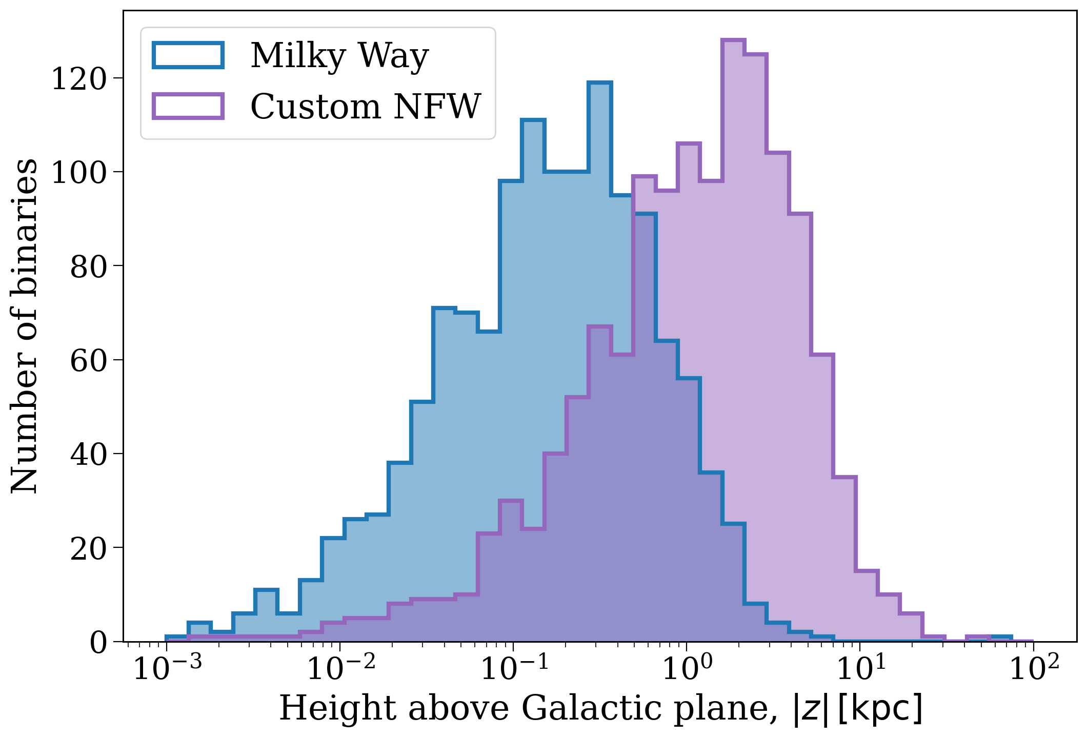
As one might expect, given the shapes of the potentials above, the custom NFW profile is less strongly bound in the $z$ direction and so we tend to find that the distribution of heights above the plane is at larger distances.

Wrap-up

Tutorial complete! Seems to me like you’ve earned a celebratory cookie. Unfortunately I’m going to have to leave it as an exercise to the reader to acquire a cookie, for now this one will have to do: 🍪.

Check out the next tutorial to learn about defining your own custom star formation histories (or do a different tutorial, or run away to the nearest beach, or whatever you like - I’m just a notebook, I can’t tell you what to do!).

Note

This tutorial was generated from a Jupyter notebook that can be found here.